
RF15-I instrument developed jointly by the Czech Astronomical Institute and the Space Research Centre of Polish Academy of Sciences is described. Methods are presented which were used to generate and reduce the modulated soft X-ray signal as expected to be measured by the instrument when in orbit. The atlas of modulated signal has been prepared. Deconvolution procedures are described and documented. Successfull launch of the INTERBALL mission took place on 3 August 1995 from Baikhonur cosmodrome.
Key words: Sun-flares-Interbol-X ray Tomograph RF15-I
The RF15-I instrument is designed to study solar flare X-ray radiation with emphasis on flare energetics. It consists of a block of detectors and the on-board computer PRAM. The block of detectors splits functionally into two parts: soft and hard X-ray photometer observing the whole disk solar emission with high time resolution and solar soft X-ray imager (KRF) called the tomograph. The tomograph unit has been designed and made entirely in the Solar Physics Division of Polish Space Research Centre in Wroclaw. Also, the on-board software related to the tomograph operations has been developed in Wroclaw. The objective of the tomograph is to image solar flare emission in two energy bands 2-4 keV and 4-8 keV by means of the numerical reconstruction of the soft X-ray signal modulated by the collimator due to the rotation of the satellite. The other components of the RF15-I instrument were designed and made in Czech Republic, under guidance of Dr. Frantisek Farnik from Astronomical Institute in Ondrejov.
The instrument has been launched from Baikonur as part of the Scientific payload of the Interball Tail Probe on 3 August 1995. Prompt analysis of the early data indicate that RF15-I instrument is in healthy conditions. The orbit of the Tail Probe is higly excentric with apogeum/perigeum of 200000/400 km and orbital period 96 hours. The satellite is rotationally stabilised; rotation period is
![]() 2 minutes. Rotation axis is to be repointed towards the centre of the solar disk periodically (once per
2 minutes. Rotation axis is to be repointed towards the centre of the solar disk periodically (once per
![]() 10 days), each time it moves by more than 10o from the Sun due to motion of the Earth around the Sun. The signals incoming from the tomograph are processed in real time by PRAM onboard computer and stored in the onboard memory. About 80 images can be stored between consecutive telemetry dumps.
10 days), each time it moves by more than 10o from the Sun due to motion of the Earth around the Sun. The signals incoming from the tomograph are processed in real time by PRAM onboard computer and stored in the onboard memory. About 80 images can be stored between consecutive telemetry dumps.
A concept of modulation collimators is bases on reconstruction of the full two-dimensional image from set of one-dimensional projections. The rotating modulation collimator has been first used in X-ray astronomy by Oda et al. (1965) to determine the angular extension of Sco X-1 source. In 1968, for the first time, the solar hard X-ray flare was localized on the solar disk using this technique (Takakura et al., 1971). Progress in technology and three-axis attitude stabilization of satellites resulted in development of the imaging collimators and telescopes with the position sensitive counters or CCD devices. However, a high-resolution images can still be obtained using low cost spin-axis-stabilized spacecrafts with a simple rotation-modulated collimator signal. One of the best examples of the result of such an experiment are the hard X-ray images of solar flares obtained from the rotating modulation collimator aboard the Japaneese satellite HINOTORI (Tsuneta, 1984).
Below we present a similar, but more advanced concept of the high-resolution tomograph X-ray imager launched aboard the Interbol satellite mission.
In the following Chapters we present a description of the tomograph construction, operation and data reduction which are essential for the reduction of real measurements. Special attention is given to description of the on-board and ground processing of the expected data. Actual codes used for this purpose are attached in the Appendixes.
The Rotating Modulation Colimator (KRF-polish acronime) consists of the two units:
X-ray collimator (XRC) optical solar disc sensor (SDS)
The purpose of XRC is to measure the X-ray signal from flares and active regions modulated due to rotation of the spacecraft. The disc sensor SDS is used to establish coordinates of the centre of the solar disc respective to the X-ray source. This will enable identification of the active region contributing to the X-ray signal.
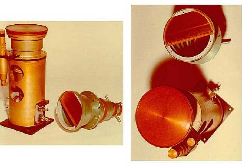
XRC consists of the 3-grid collimato (see photographs) placed in front of the double proportional counter operating in the 2-4 keV and 4-8 keV energy range. Due to rotation of the satellite, X-ray radiation emitted by flare or the active region passes through different portions of the collimator, depending on the phase of the rotation. The collimator's field of view has radius of 10o.8 , and has a number of narrow (
![]() 11 arcsec) transmission windows separated by 4.8 arcmin. Grids are made of cooper wires of 66.8 microns diameter placed exactly parallel within a distance of 75 microns. The exact location of the grids have been calculated according to the novell strategy developed by Kordylewski (1988) which allowed to use only three grids instead of four which would be necessary in
11 arcsec) transmission windows separated by 4.8 arcmin. Grids are made of cooper wires of 66.8 microns diameter placed exactly parallel within a distance of 75 microns. The exact location of the grids have been calculated according to the novell strategy developed by Kordylewski (1988) which allowed to use only three grids instead of four which would be necessary in
Fig. 1
Scheme of the X-ray collimator. The front grid consists of the three areas: transparent (no grids), the diagonal bar stopping completly the radiation and the gridded half. Central grid is also partly transparent, matching the front one. The end grid located immediatly in front of the double proportional counter is fully covered by grids. The distances between grids has been optimized in order to create repeated pattern of transparent triangular field of viewsthe classical approach (Nobles et al., 1980). The front and the middle grids cover only approximately half of the conica field of view. The front grid has a special occultation strip allowing to measure ''background'' signal. The last grid covers the whole aperture. This special arrangement of the grids allows for the soft X-ray radiation emitted by solar source to be modulated due to rotation of the satellite (as shown in the Fig. 2). The number of transmission strips depends on the actual pointing of the satellite rotation axis relative to the centre of the solar disc, location of the source on the disc, etc. The position of the satellite rotation axis relative to the ''optical'' Sun is monitored by the SDS unit. It consists of the optical system which image the solar disc on the system of two narrow slits, coaligned with the optical plane of the X-ray collimator as shown schematically in Fig. 3. Rotation of the spacecraft causes the optical disc to circle through slits and the modulation of the intensity of the radiation passing through the slits takes place. This intensity is monitored by the photodiode located behind the slits. Instant values of the solar position phase angle and the offset of the rotation axis are calculated by the on-board computer PRAM from the history of slit cross timing of the previous rotation.
The data gather time unit is 1/128 s for the X-ray detector while outside the radiation belts. During belt crossing the high voltage is turned off from the detector.
After full revolution of the spacecraft in ''normal'' conditions, the following information is collected:
The signals coming from both low and high energy channels are processed in real time by the PRAM computer and depending on the level of the signal, memory available, etc. (as discussed in detail in Sections 4 and 4.1) decision is made whether to store the modulated signal (about 10 kbytes) to the memory for image reconstruction on the ground. If so, before being stored, the information is compressed and periods when the source is outside narrow fields of wiev are discarded. Generally our intention is that for each flare of the GOES class above C5, at least one sequence of modulated signal will be recorded, usually at the flare maximum when the time variation of the signal influence the image restoration process least. Average unmodulated signals from both energy channels are recorded once per revolution.

Fig. 2
Schematic drawing showing various phases of the modulation of the solar radiation in the collimator. The Sun is shown as a small circle with the X-ray source as a small spot. Due to rotation of the spacecraft the apparent position of the source as seen from the position of the detector window follow the circular path. For less than half of the rotation period (phase a) no modulation of the signal is observed. At phase b the source enters the occultation stip which angular width is more than the solar diameter and therefore, at phase c, the solar soft x-ray radiation is totally dlocked and the signal corresponds to detector background. At phase d the source enters the gridded section of the collimator and the signal is modulated when the source crosses individual transmission windows. At each transmission window, the X-ray source is scanned at different angle (changing by p/2 between phases d and f).
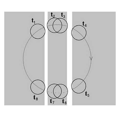
Fig. 3
Scheme of the ''motion'' of the visible image of the solar disc across the system of the slits in the SDS unit. At time t1-t8 the electronic system connectedfields of view are discarded. Generally our intention is that for each flare of the GOES class above C5, at least one sequence of modulated signal will be recorded, usually at the flare maximum when the time variation of the signal influence the image restoration process least. A verage unmodulated signals from both energy channels are recorded once per revolution.
In order to better understand the form of the signal to be registered during passage of the source through the modulation zone of the collimator we have performed the task of numerical simulation of the form of the signal for various combinations of the source geometry and relative offset of the source from the direction of spacecraft rotation axis. In particular, we selected the following set of geometry for the sources:
The simulations were performed for various values of the offset between the source and direction of the rotation axis of the spacecraft d. In the simulations we have adopted the following values of the important parameters:
For detailed description of the X-ray detector used in the experiment see Sylwester and Farnik (1990). In calculating the effective collimator transmission allowance had been made for effects of diffraction still important for the soft X-rays because of the very narrow slits in the collimator grids (Kordylewski, 1994). In the simulations we assumed that the source total intensity corresponds to the flux of about 106 photons/cm2/keV/s at Earth (GOES M flare). In Fig. 4 we illustrate the form of the signal coming from the single source (compact flare) having the conical intensity distribution of FWHM = 10 arcsec for case when d = 6o.

Fig. 4:
Example of the KRF signal from a simple conical source of 10 arcsec FWHM in case when the rotation axis of the satellite is pointed d = 6o off the source. In the upper panel individual phases of rotation are designated according to Fig. 2. The middle and lower panel shows enlargements of the selected portions from the upper panel. In Figs 4- 16 the statistical noise has been introduced assuming Poisson count statistics and detector background of 6 counts/s.In Figs 5-8 we show, how the form of the signal (from the same source as in Fig. 4) depends on the offset d. For d < 0o.54 as in Fig. 5, the signal is modulated all the time and the source doesn't cross the occultation bar. In Fig. 6, the case is illustrated when the source enter the occultation strip only once during the rotation. Fig. 7 and 8 give examples of the record to be seen around 4th and 10th day after repointing the satellite, when d = 4o or 10o. All phases of the modulated signal are present in Figs 4,7 and 8 (a, b, c, d, e and f in Fig. 2)

Fig. 6:
Same as in Fig. 4 For the offsetd= 3o .
Figs 9-11 demonstrate the modulation of the signal for assumed double source (e.g. flaring loop footpoints, d = 6o) with various seperation of the sources (5, 10, 20sec respectively). It is seen that even for the separation of 5sec the signal is of double peak form and both sources can be resolved on the restored image.


Fig. 11:
Same as in Fig.9 for the emission centers separated by 20 arcsec.Fig. 12 demonstrates the case when the source consists of many subsources resembling the whole loop-like structure (also for d = 6o)

Fig. 12:
Example of the signal modulation for the configuration of 5 sources resembling the loop-like flaring structure.Figs 13-16 show the effect of varying angle q between the line connecting the double source and the collimator plane (0o, 30o, 60o, 90o) has been selected and the intensity ratio between the sources is 2 : 1.d = 6o and sources separation is 30sec in this simulations. Depending on the q value the double structure on the modulated record manifest itself at different portions (phases) during the rotation.
Fig. 13:
Examples of the dependence of the modulated signal on the relative phase of the second source relative to the first.(Data on parameters). It is seen that the double structure of the transmission peaks arrives at different fingers on the record.
Fig. 14:
Same as in Fig. 13 for relative phase 30 o.
Fig. 15:
Same as in Fig. 13 for relative phase 60 o .
Fig. 16:
Same as in Fig. 13 for relative phase 90o.0The examples shown above (Figs 4-16) and results of numerous other simulations performed consist of the Atlas of KRF records. This Atlas will be usefull in a fast identification of the nature of the source from ''raw'' measurements.
The data from the KRF sensors are to be processed by the program contained in the EPROM memory within the PRAM comupter. The name of the program is KRF and has been written in assembler language for the NSC600 processor. Writing the program we have had to take into account the following limitations:
The above limitations (especially items 4 and 6) forced, that the structure of the data interpretation algorithm and organization of the data transfer to the recorder is very complicated. In addition, to save the memory, the algorithms cut-off portions of constant signal. Data from X-ray detector are constantly monitored in order to detect the flare, estimate its class and decide when and which observing sequence has to be executed. The data from optical sensor are dumped to the recorder after each 100 sequences (rotations) while the data from X-ray detector are transmitted in the following modes:
Such organization of the data transfer substantially compress the volume of the data to be recorded, but necesserily needs the time from the onboard clock to be assigned to each data pack. To shorten the time info, the ''local clock'' has been introduced (giving the pack No in a sequence).
The activity level is determined by comparing the X-ray signal with the threshold levels which are modified depending on: the memory quota available on the recorder, the history of solar activity and after each 30 rotations. In the next subsection we give more details on the KRF programm structure and the printout of the algorithm is given in the Appendix 9.2.
The scientific part of data block is divided into 7 frames, each 16 bytes long. Following the reset of the power and after each 100 measurement cycles
(one cyle = rotational period), 2 measurement cycles are devoted to record data from optical sensor (32 bytes). For other mesurement cycles the following data are recorded artelnatively:


 |
 |
|
|
|
| BACK | HOME PAGE CBK |
File translated from TEX by TTH, version 1.57.