 |
We present the iterative deconvolution algorithm called ANDRIL devoted for advanced processing of images obtained by the Soft X-ray Telescope (SXT) on Yohkoh. The algorithm is based on maximum likelihood approach. We introduced several modifications to this algorithm in order to optimize its properties. The goal of the algorithm is to remove numerically the image blurring due to the instrument point spread function (PSF) and increase the image resolution. The application of the algorithm allows to resolve soft X-ray structures on the SXT images on the angular scales down to 1 arcsec. Presented algorithm is being used recently for analysis of detailed morphology and physical conditions in the plasma of flaring structures.
Key words: Sun: X-ray-SXT-image processing
Most of the physical processes responsible for energy release in the corona are supposed to act on very small scale lengths, below the resolution of Yohkoh Soft X-ray Telescope (SXT). However, the fact that the pixel dimension and full width at half maximum (FWHM) of point spread function (PSF) for the grazing incidence mirror are of similar size offers the possibility to ''enhance'' the effective resolution using image reconstruction techniques. In a number of recently published articles (Karovska and Hudson 1994, Roumeliotis 1995, Alexander and Metcalf 1997, Magain, Coubrin and Sohy 1998) methods are discussed which allow to restore and/or increase numerically the resolution of the restored images by adopting diverse approaches: blind search, modified maximum likelihood method and pixon cells. Results of these investigations suggest that appropriate image reconstruction algorithms do offer the possibility to increase spatial resolution of the SXT by numerically removing the instrumental blurring. Based on the experience acquired related to integral inversion techniques in one, two and three dimensions we have developed fast deconvolution algorithm specially designed for purpose of massive SXT image processing. Below we present basic formulation of the maximum likelihood reconstruction algorithm (following White 1993), discuss adaptations introduced in order to use it for massive processing of the SXT images and present example results of numerical tests. The test results obtained indicate what are advantages/disadvantages of applying presented algorithm for reconstruction of the detailed morphology of X-ray emitting structures. The example of deconvolution for real SXT flare images are presented.
Based on our previous experience with iterative algorithms (in one dimension - DEMON: Withbroe 1975, Sylwester, Schrijver and Mewe 1980, Fludra and Sylwester 1986, in three dimensions: Pres, Siarkowski and Sylwester 1995) we came to the idea of adopting DEMON multiplicative algorithm for two-dimensional task of image enhancement. Incidentally, during the adaptation it turned out that DEMON algorithm directly corresponds to Richardson-Lucy (R-L) method of image enhancement which received substantial attention in relation with attempts of numerical correction of early Hubble Space Telescope images.
The R-L iteration condition can be derived (Richardson 1972, Lucy 1974, 1995, White 1993, 1994) assuming the Poisson probability distribution of the signal forming the image:
 |
Here P(N |`N) is the probability of getting N counts in a pixel when the mean expected number of counts is [`N], and the ''convolution'' equation is:
 |
where f is the unknown source brightness distribution, P( i | j ) is the PSF (the fraction of light coming from the true location ''j'' that gets scattered into the observed pixel ''i'') and C is the blurred image. If PSF does not vary with position in the image then P( i | j ) = P( i - j ) and the sum becomes a ''true'' convolution. As discussed in Section 3.1 SXT PSF varies with the position, but locally can be assumed as constant. The joint likelihood L of getting the observed counts Oi in the pixel ''i'' given the expected counts Ci is:

The maximum likelihood solution occurs when all partial derivatives of L with respect to fj are zero which leads to the following iterative multiplication condition:

The correction factor Oi/Ci approaches unity as the iteration proceeds and fnew converges to the maximum likelihood solution as has been proven by Shepp and Vardi (1982).
The standard R-L method has a number of characteristics which make it well-suited for purposes of image reconstruction ( White 1994):
The examples of image reconstruction obtained using standard R-L algorithm for four synthetic test sources are shown in Fig. 1. Each pixel has been sub-divided into array of 5 x 5 sub-pixels. In the left column the test model is presented within the area of 100 x 100 sub-pixels (20 x 20 SXT pixel area). The middle column represents the corresponding input image that would be observed by SXT using Al01 filter provided the region is located close to the western solar limb. The right column represents the image restored after 50 steps of iteration. In the test model we have assumed that the bright features have the width of one sub-pixel, and constant intensity (1000 counts per sub-pixel). The level of background is assumed to be 10 counts/sub-pixel. The statistical noise has not been taken into account in these examples for clarity. Extended discussion of the noise influence on the results of image deconvolution will be discussed in a dedicated paper (Sylwester & Sylwester, 1998).
In the iteration procedure we assumed (here and
generally in all the other cases) flat distribution as the ''zero
approximation'' for f. In order to
handle the boundary regions, we artificially extended the working
arrays by the width of the PSF field array and filled this added
region with the intensity equal to the average from the outermost
input pixels (as taken from the middle image). This necessarily
introduces some freedom which sometimes manifests itself as
presence of unexpected, relatively small ''edge features'' (third
row in Fig. 1). The comparison of input (middle column) and
R-L restored images (right column)
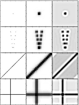 fig1.ps.gz(30k)
In the rest of this Chapter we will discuss the modifications which we have implemented into to R-L algorithm in order to improve its image reconstruction characteristics.
One of the disadvantages of R-L algorithm is the amplification of the noise present in the actual data. White (1994) proposed the modification of the likelihood function as expressed by Eq. (3) in order to damp the influence of statistical noise present in the data. He reasoned that if the difference between the blurred model (C) and the observations (O) is large compared with the uncertainties, the use of likelihood function as in Eq. (3) is justified. However if this difference is smaller than the noise he suggested to use modified likelihood function. The modification makes the likelihood function flatter in the vicinity of a good fit. Here for completeness, we recall formulations of the damped iteration.
''Damping function'' f(x) introduced by White
is of the form:


Using this new likelihood function one can
derive the following expression for R-L damped iteration:

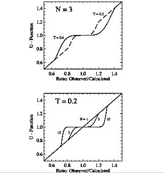
The constant N determines how suddenly the function f(x) becomes flat for x < 1. For N = 1, f(x) = x and there is no flattening at all and the iteration is exactly the same as in the standard R-L algorithm. Otherwise, for N > 1, in the regions where the differences between observations and the model are small compared with the noise, the U function damps corrections of the model. U function has a continuous first and second derivative which is important since R-L algorithm ''dislikes'' discontinuities. The influence of damping on the noise pattern is illustrated in Fig. 3. The reconstructed images for selected combinations of N and T are shown together with ''no damping'' case (upper left). Presence of statistical Poisson noise has been assumed in the synthetic model. As pointed out by White (1994) the larger is the value of T, the smaller is the noise due to statistical fluctuations present in the data. One may observe that using the damping function U reduces also the influence of ''ringing''. The results reported in the rest of this paper (where appropriate) correspond to N = 3 and T = 0.2 which values compromise the smoothing influence of the U function with the ability to restore localized sources in case of SXT deconvolution.
Several researches (cf. White 1994) discovered
independently a technique for accelerating the R-L method. The
basic idea is that within given iteration step the search is
performed for such value of the parameter A (the same for all
pixels)
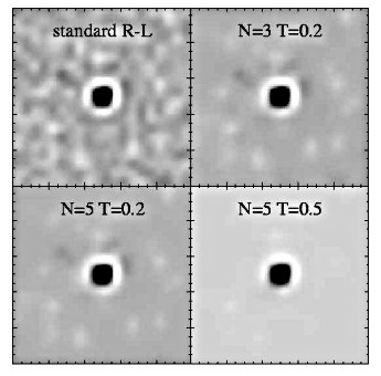 fig3.ps.gz(22k)
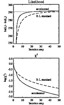 fig4.ps.gz(4k)
 Figure
4: Likelihood L (upper part) and c2 (lower part) convergence of
the standard R-L (dashed) and accelerated (continuous)
iterations.
the convergence of the likelihood is illustrated as defined in
Eq. (3). In the bottom part we compare behaviour of the c2 value. The c2
value plotted corresponds to this portion of the image where the
relative uncertainty of the signal is better than 20%, i.e. where
the observed signal is above 25. We applied this 20% criterion
for calculating c2
consistently in the rest of this paper. Selection of such
criterion reflects our choice of the value for T parameter.
It is seen from Fig. 4 that acceleration indeed speeds up the convergence, and the value reached in 50th iteration step in the standard method is obtained in 20th iteration in the accelerated approach. The actual increase of L in the last iteration step amounts to ~ 1. The final value of maximum likelihood obtained within the accelerated scheme is by 2.6 higher than in the standard approach. Also the final c2 value is in the accelerated case factor of four lower than in the standard approach. In most cases the increase in L is accompanied by decrease of c2. However accelerated scheme may sometimes result in the situation when the L value still increases while c2 begins to increase slightly. This may happen since the method is derived from the condition of likelihood maximization - not c2 minimization. Anyhow the increase of c2 is not large and amounts to few percent in these cases. A good property of the accelerated algorithm is that it converges to the final, well defined solution after 35�50 iteration steps (Table 2). This is not the case for standard iteration scheme where it is necessary to set criterion when the iterations should be terminated.
We have investigated how the results of deconvolution depend on the number of pixel sub-division. In Fig. 5 we present example results which have been obtained for the point source located in the centre of FOV for various number of sub-division schemes.
Based on these results and for the other source configurations tested, we decided to run SXT deconvolution using the sub-division of each pixel into 5 x 5 sub-pixels in massive calculations. The results obtained do not differ substantially between 3, 5 and 9 sub-divisions. The same choice of 5 sub-divisions has been made by Roumeliotis (1995) and it is in agreement with note of Martens, Lemen and Acton (1995). By adopting 5 x 5 sub-division scheme it is possible to locate point-like sources with the precision of ~ 0.5 arcsec.
While restoring images obtained by means of
CCD, standard problem arises for regions with low signal. Often,
following the dark current subtraction, the resulting signal is
negative since the dark current information is in most cases a
time-interpolated guess only and the signal itself statistically
fluctuates. Dealing with negative signal is very inconvenient
within always positive algorithm like R-L. Usually one has to
adopt some positive value for these negative numbers.
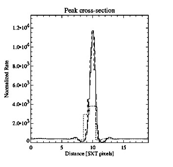 fig5.ps.gz(5k)
 Figure
5: Horizontal-cut profiles of the deconvolved image (Al01
filter) of the point like source located exactly at the centre of
FOV for four sub-division selections. Dotted line represent 1:1
case (no sub-division), short dashed, continuous and long dashed,
1:3, 1:5 and 1:9 cases respectively.
However, the dynamic range and smoothness of the solution depend
critically on this adopted positive value making the solution
subjective close to regions of small signal. In order to find the
solution to this problem we modified the iterative condition (4)
in the following way:

This section completes description of the modifications which have been made to the Richardson-Lucy algorithm in order to improve its characteristic. We call the improved algorithm ANDRIL (Accelerated Noise-Damped Richardson-Lucy). Based on the numerous tests performed, we have found that it always converges in terms of increasing the likelihood characteristic. In most cases the method approaches the limit before 50th iteration step which (otherwise) we selected to be the final step. In case when substantial statistical noise is present in the data, stopping the convergence when c2 � 1 prevents fitting the noise (see discussion in Sylwester and Sylwester 1998).
It is worth to note that the described algorithm can be used in order to restore images in the case when instrumental PSF is of peculiar, very asymmetric shape. This has been shown in Fig. 6 for the adopted PSF of L letter shape, with the arms inclined relative to the observational net. For such PSF the observed image only barely resembles the shape of the source. However the restored image represents the model source shape closely.
The example shown indicates that the algorithm can be applied in order to restore images obtained using quite asymmetric PSFs.
One of the main characteristics of the image reconstruction method is its ability to restore the real intensity pattern. As mentioned before, in case of the sources with the strong gradients present (Fig. 1), the intensity distribution on the reconstructed image may substantially differ (tens of percent) from the original even in case when the formal fit between the ''input'' and reconstructed image patterns is exact. This is due to the ill-conditioned nature of the reconstruction problem. In Fig. 7 we illustrate this effect in more detail.
In case of discontinuity present on model image
(continuous line in Fig. 7a) the reconstructed image (dotted
line) tends to fit the model distribution well except the region
of a sharp gradients (around 10th pixel). The edge
artifacts are also noticeable. The steep gradient is smoothed
within two pixels around the discontinuity. One observes
over/under shooting by up to 10% surrounding the discontinuity.
The width of the ''smoothed'' region can amount to few
sub-pixels. One has to remember this property of the method when
interpreting the results of real images deconvolution. For
smoothed model distributions (continuous line in Fig. 7b),
discrepancies between the original and restored shapes tend to be
smaller. In the example shown,
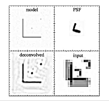 fig6.ps.gz(15k)
 Figure 6:
ANDRIL deconvolution exercise for artificial PSF function of
highly asymmetric shape. In the upper left frame the assumed
model is presented. Upper right frame presents the shape of PSF.
Lower right frame is the input image for deconvolution (as would
be observed for such PSF) while the lower left frame is the
deconvolved image.
the FWHM of the restored structure is the same as for the input
distribution (1.3 SXT pixel). Note that the ''ringing'' is much
smaller in this example than in Fig. 1 since we have used
damped approach in this case.
In order to look in more detail into the ''intensity pattern'' reconstruction, we performed another exercises. First, we assumed that the source consists of many smoothed, point-like sources arranged along the diagonal line at various distances in between. The intensities of the sources vary in proportion to the position along the diagonal, as shown in Fig. 8.
Another example is shown in Fig. 9, where two diagonal line sources cross in the middle.
In Fig. 10, we illustrate how the
reconstructed pattern depends on the ratio of signal to noise.
Here we consider three cases when the contrast between the
maximum and noisy background signals is 80, 8 and 2 respectively
on the input (model convolved with PSF) image.
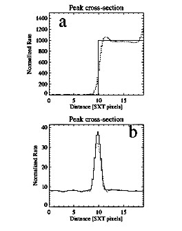 fig7.ps.gz(3k)
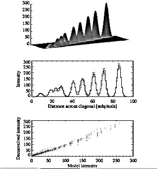 fig8.ps.gz(42k)
 Figure
8: The results of ANDRIL image restoration for the test
source consisting of many smoothed point-like sources arranged
along diagonal line. Upper - assumed shape of the test sources.
The intensities of individual components are proportional to
their position along diagonal. Middle - comparison of the model
(continuous) and restored (dotted) intensity profile along the
diagonal. Lower - correlation plot of the ''deconvolved'' image
intensities plotted against the model for all sub-pixels
including these representing noisy background. The intensity
units are counts per sub-pixel.
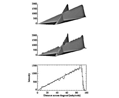 fig9.ps.gz(34k)
 Figure
9: The results of ANDRIL image restoration for the test
source consisting of two crossing linear smoothed structures.
Upper - the shape of the input test image where intensities are
proportional to their positions along diagonal. Middle - restored
shape.Lower - comparison of the model (thin) and restored (thick)
intensity profiles along one diagonal. The intensity units are
counts per sub-pixel.
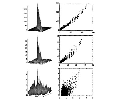 fig10.ps.gz(411k)
 Figure 10:
Dependence between the restored and model intensities
(DN/sub-pixel) on the contrast of the brightest observed feature
and the noisy background. The left column presents the shape of
restored image as expressed in counts/sub-pixel. The test source
shape is the same as shown in Fig. 8. The right column shows
correlation plots of the model intensities (horizontal axis) and
restored intensities (vertical axis). The three rows represent
cases when the contrast between the brightest element in the
observed (input) image and the background is 80, 8 and 2 (from
the top to bottom respectively).
It is seen that there is a tendency for restored maxima to be 10% � 30% higher than for adopted model. Otherwise the correlation is good except the region of very low signal (less than 2 counts/sub-pixel) where the correlation is lost. However even in case of low contrast, the strongest sources present in the model are restored well, not only as concerns position, but also the intensity. This result is encouraging. However, calculated brightness distribution is sensitive to the presence of data noise. The amplitude of the noise (relative to the signal) in the deconvolved image is about factor of four larger than the relative amplitude of noise in the data itself. In a separate paper (Sylwester and Sylwester 1998) we will address this problem in more detail and examine ways haw to overcome the noise amplification.
The tests performed and illustated in Figs 7�10 show that:
The above described algorithm has been coded using IDL programming language (double precision). It consists of several subroutines. In Table 1 we present the dependence of the computer time necessary to perform SXT deconvolution on the sub-division scheme and dimension of PSF array. Since most of the flare image sequences obtained by SXT cover area of 64 x 64 pixels, we run our time-test exercises for such a region.
Table 1: Time necessary to complete ANDRIL image restoration
Pixel Sub-division |
5 |
PSF size 7 |
13 |
1 |
0.14 |
0.15 |
0.16 |
3 |
0.41 |
0.41 |
0.48 |
5 |
0.98 |
1a |
1.41 |
7 |
2.93 |
3.13 |
4.50 |
aThe unit corresponds to 55 min of Sun-Sparc 20 workstation CPU.
Inspection of the Table indicates that the selection we have made in order to deconvolved SXT images (division of the pixel into 5 x 5 sub-pixel elements, and use of 7 x 7 pixels PSF FOV) constitutes a reasonable compromise also in terms of CPU time. Changing from 5 x 5 to 7 x 7 pixels PSF FOV does not increase CPU time substantially.
The Soft X-ray telescope operating aboard the Yohkoh is yet the most successful solar X-ray mission. It has been developed by USA/Japanese consortium (Tsuneta at al. 1991). By now it has registered millions of solar images related to such solar phenomena as coronal holes, bright points, active regions, flares and coronal transients.
The instrument consists of the grazing incidence modified Volter II type mirror, rotating wheels with various filters and the CCD detector at the focus. Within particular observing sequence various filters are being interchangeably inserted into the solar X-ray beam allowing to obtain images in slightly different energy portions of the soft X-ray spectra.
It is necessary to understand a number of peculiar characteristics of the SXT instrument and data reduction in order to make appropriate tailoring of the maximum-likelihood image restoration algorithm.
The point spread function of SXT has been analysed by Martens, Lemen and Acton (1994) based on the results of ground calibrations. They have found that it can be well approximated by an elliptical Moffat function (Bendinelli 1991) of the form:

Weston and Acton (1996) investigated the dependence of PSF shape on the average energy (temperature) of the incoming radiation and provided the plots of the temperature dependence of ''a'' parameter. In the present paper we have used the PSF as can be calculated from the IDL SXT library routine SXT_PSF written by Barry LaBonte (cf. SXT software) and modified in order to allow for over-resolution and double precision calculations.
For given location on the Sun, we have assumed that PSF shape is constant within the FOV framing the flare (64 x 64 pixels). Such assumption speeds up enormously the calculations and is justified since the relative change of the shape is less than 5% between the centre and the corners of SXT frame. The Moffat approximation used for PSF calculations may be slightly different from the actual shape of the PSF (as discussed in Sylwester, J., Sylwester, B. and Siarkowski 1996). In order to find a reasonable compromise between the size of the PSF which is used in the deconvolution process and the computation time, we performed calculations on selected SXT flare image (Fig. 15) for a set of PSF arrays cropped within 3, 5, 7 and 13 SXT pixels. In Table 2 we present final converged quality characteristics of the runs.
PSF size > |
3 |
5 |
7 |
7a |
13 |
iteration |
44 |
38 |
40 |
46 |
42 |
lnL |
301134 |
301099 |
301072 |
300951 |
300864 |
c2 |
0.0506 |
0.0560 |
0.0573 |
0.239 |
0.1108 |
The FWHM of PSF is ˜
1 SXT pixel, so the actual size of the PSF area used
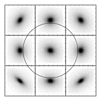 fig11.ps.gz(18k)
 Figure 11:
Schematic picture indicating changes of the PSF shape for
different locations of boxes relative to the solar disk. The
centres of individual frames point to the appropriate positions
relative to the solar disc (circle). The size of each box is
7 x 7 SXT pixels (note that the size of solar disc is
not to scale).
in calculations should be several times larger. The values in
Table 2 reveal that the larger is PSF area, the worse is the
final fit (decreasing L and increasing c2
trends with increasing size). This indicates that the shape of
the PSF in the far wings as taken from Moffat approximation might
be somewhat uncertain. However, this difference does not
influence substantially the results of deconvolution for
relatively compact intense sources like flares as is shown in the
next example.
Inspection of the shapes of image deconvolved with differently sized PSF indicates that the larger is size of PSF area, the smoother and less noisy are the results. The choice of 7 x 7 pixel area for PSF represents a compromise selection for massive SXT deconvolution task.
It should be noted that results of the
deconvolution are not strongly dependent on the possible
uncertainties in the PSF shape. In Fig. 12 we compare
deconvolved
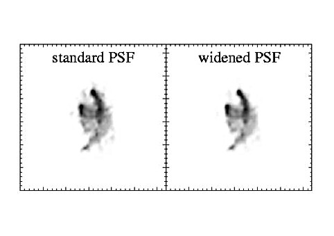 fig12.ps.gz(28k)
 Figure
12: Comparison of the deconvolved images for standard and
artificially widened PSF. The size of PSF area has been taken as
7 x 7 pixels in both cases.
images obtained for ''standard'' PSF as calculated from Moffat
approximation and the different, wider PSF taken as the
''standard'' raised to the 0.8th power. In this way
the corresponding increase of the PSF FWHM is 20%, central peak
value is 1.5 times lower and the far wings are twice increased in
intensity.
It is seen that such modification of the PSF FWHM does not substantially change the deconvolved pattern except that the bright sources become 30% more intense, their widths decrease by 10% and some weak sources disappear. In Table 2, we put corresponding best fit values of L and c2 obtained for this run (subscript a). Forced change of PSF shape worsen substantially the final fit characteristics.
The images recorded by SXT are expressed in so-called data numbers (DN) which reflect the X-ray photon fluxes in rather complicated way, depending on the photon energy. In order to avoid problems with negative count rates we have applied the approach discussed in Section 2.4 (we deconvolved the images based on direct decompressed measurements, adding the ''dark current'' at the appropriate place within the code).
Below we consider in more detail two of the effects which are the most important for image restoration namely the conversion of DN to the photon number and estimation of the measurement uncertainties.
Each energy channel of SXT (filter combination)
has different overall sensitivity to the incoming spectrum of
X-ray photons (depending on the spectral shape i.e. source plasma
temperature). By itself this means that the conversion of DN to
photon depends on the source plasma temperature. Using the
routine SXT_FLUX (Yohkoh Analysis Guide, 1994,
p. 19) one can examine this dependence. We have plotted it
in Fig. 13. Based on these data one can determine values of
average conversion factors DN/photons for source plasma from the
temperature range 4�20 MK. We
derived these averages to be: 3.02, 3.14, 5.59, 3.54 and 3.00 for
SXT filters Al01, AlMg, Be119, Al12 and Mg03 respectively. These
average values have been used to convert DNs to photons in order
to calculate the appropriate uncertainties.
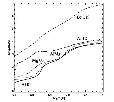 fig13.ps.gz(3k)
There are at least three sources of uncertainties which contribute to total uncertainty of the SXT DN signal:
We used quasi Monte-Carlo approach in order to estimate the common effect of them. We generated a sequence of numbers covering the entire range of valid (unsaturated) CCD signals (up to 3300 DNs). Each value of the signal has been converted to corresponding photon number ( N) perturbed randomly assuming Poisson character of the signal (s ~ �{ N}), compressed and decompressed. The unperturbed signal has been subtracted from the decompressed perturbed signal. This difference, after averaging over the perturbed set has the sense of combined statistical and compression/decompression uncertainty. The uncertainty of dark current signal (as estimated from interpolation between preceding and following in time dark frames) has been again assumed to have the statistical character. In Fig. 14 we plot the log of overall relative uncertainty [(D(DN))/ DN] against the value of the compressed signal.
These relative error estimates have been used
in massive SXT image deconvolution project.
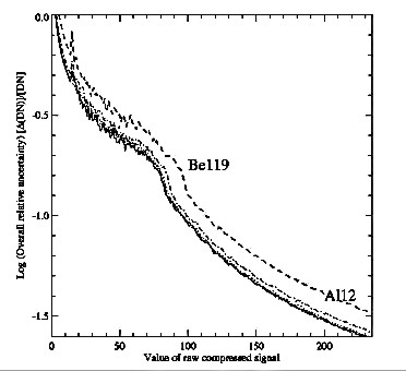 fig14.ps.gz(19k)
 Figure
14: Dependence of the log of relative uncertainties [(D(DN))/ DN] on the value of compressed
signal for individual filters of SXT. For all filters except
Be119 the lines overlap.
The automatic exposure selection scheme applied in Yohkoh SXT caused that the exposure time has been automatically reduced with increasing intensity of the flare in order to avoid pixel saturation. This exposure reduction caused the non-flaring parts of the active region (those, for which the intensity does not change substantially during the event) contribute less and less photons to the total signal (in proportion with the reduction of exposure time). Therefore the relative statistical uncertainties for these regions substantially increase, and many of the weak pre-flare features actually disappear at the times of high flare signal. One should keep in mind this effect when interpreting sequences of flaring images taken with different exposures. The problem is partly avoided while comparing frames obtained with the same exposures.
In Fig. 15 we show example of the image
restoration for real SXT observations. In the upper row we put
three compressed images obtained close in time through different
filters for flare in progress located near the western solar
limb.
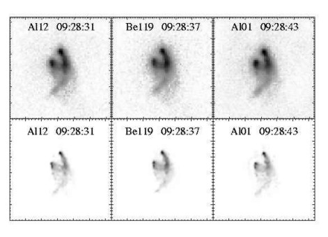 fig15.ps.gz(48k)
 Figure
15: Results of deconvolution of SXT images for flare
observed close to the solar limb on 19 November 1991. In the
upper row compressed images are shown, directly as observed. In
the lower row corresponding results of ANDRIL deconvolution are
shown compressed in a similar way. The FOV is 64 x 64
SXT pixels (156 arcsec x 156 arcsec).
Inspection of the Figure indicates that deconvolution brought up a lot of details not directly seen in the original. Pronounced are fine structures at the foot-points of the extended double loop. Number of secondary low intensity filaments are seen below the main loop and the ridge going down from the summit kernel shows up its detailed structure. The overall similarity of the details seen on all three deconvolved images strongly indicates for their physical nature.
Preliminary studies of sequences of deconvolved SXT images for individual flares and active regions have been presented by Sylwester B. and Sylwester J. (1997, 1998).
This paper introduces the maximum likelihood code ANDRIL which is being used for massive image processing of Yohkoh SXT images. The code has been developed by incorporating most of the ideas worked out for Hubble Space Telescope image restoration project. The algorithm has been developed entirely in Wroclaw having in view its application for deconvolution of extended sources like those present in solar corona. Special attention has been allocated to investigation of the application of ''over-resolution'' which allows to increase numerically the resolution on the SXT images. Extensive tests indicate that it is feasible to increase the spatial resolution in this way. A new approach has been used in order to properly accommodate the measurement uncertainties of SXT observations. The properties of ANDRIL algorithm can be adjusted to this particular task by setting the appropriate values of parameters regulating the behaviour of the convergence and smoothness of the solution. We have found that the optimum results are obtained by using the following set of parameters (discussed in details in the paper):
The use of accelerated approach speeds up the convergence by factor of about 3�5 and causes the solution to reach the asymptotic value after 35�45 iterations. Results of numerous tests of the algorithm indicate that modified R-L deconvolution algorithm can be successfully used in order to remove the SXT PSF and bring up details on the images with the size down to ~ 1cases the intensity pattern obtained in the deconvolution process constitutes the actual intensity pattern in the source. It should be noted however, that some uncertainty exists in regions where strong gradients are present. There is definite pattern indicating that the derived intensities of well-localized sources are higher by 10%-20% than in reality. The deconvolution close to the edge of the observed field of view may be somewhat uncertain due to ''edge artifacts''.
In spite of these well identified and tested shortcomings of the present algorithm, the application of ANDRIL reveals many new fine structures in the SXT images. Their physical reliability is confirmed when analyzing the time sequences of deconvolved images and from the comparison of deconvolved images obtained using different filters (for close in time exposures). By now, the inspection of many such sequences led to development of a new concept of hierarchical model describing the organization of magnetic fields in the corona (Sylwester J. and Sylwester B. 1997).
The ANDRIL code will soon be available as the IDL package on request.
Acknowledgments. We would like to thank the referee for helpfull suggestions which led to the improvement of this contribution and inspired the following one. This work has been supported by Polish KBN grant 2.P03D.006.10.
File translated from TEX by TTH, version 1.57.