ESA SP-506 Vol. 2, p. 769-772, 2002
MULTITEMPERATURE ANALYSIS OF SELECTED LIMB-OCCULTED FLARES
Space Research Center, Polish Academy of Sciences, Wroclaw, Poland
ABSTRACT
The aim of this contribution was to compare the so-called " quasi" differential emission measure distributions (qDEM) with a "classical" DEM distributions. The qDEM distributions for the flaring region have been derived from the maps of "isothermal" temperatures and emission measures for the flaring region. The temperature and emission measure maps have been derived based on the deconvolved Yohkoh SXT images. The deconvolution has been performed in order to increase the spatial resolution. Next the images have been overlaid precisely using the position of the occulting solar disc as a reference. The high accuracy of coalignmet allowed to derive the temperature maps with spatial resolution down to ~1 arc-sec. From the other side the DEM distributions have been determined for a flare as a whole, based on integral flare fluxes measured by SXT and GOES using maximum likelihood iterative algorithm. In principle such a comparison of qDEM and DEM shapes should allow to investigate which part of DEM is related to the bright kernels observed on SXT images.
Key words: Sun; flares; multitemperature plasma.
1. INTRODUCTION
In the paper by Sylwester and Sylwester (2002a) we have proposed additional technique of analysis of the distribution of plasma with the temperature for individual flaring regions. This method (called qDEM - quasi Differential Emission Measure analysis) is based on interpretation of the temperature and emission measure maps as calculated using filter ratio technique in an isothermal approximation. Classically, the multitemperature analysis of X-ray emission have been investigated in the framework of an approach called differential emission measure distributions (DEM). The references to the appropriate papers and detailed description of the algorithm leading to calculate the DEM distribution and adopted in the present contribution one can find in the paper by Sylwester et al., (1980). We will refer to this algorithm as Withbroe-Sylwester (WS). The comparison of WS and the other standard methods commonly used for DEM calculations has been discussed by Fludra and Sylwester (1986).
Here we attempt to compare the results of two methods of analysis the plasma temperature distribution using the flare SXT observations by Yohkoh and GOES. In principle the comparison of qDEM and DEM shapes should allow to investigate which part of DEM is responsible for the bright flare kernels observed on SXT images.
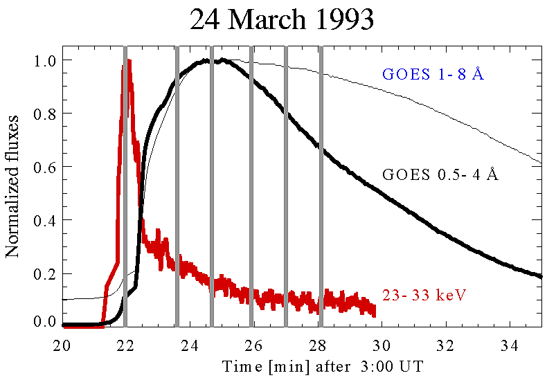
We have based our analysis on the observations of C6.6 limb flare from 24 March 1993 at 03:25 UT. In Figure 1 the three lightcurves (pair of GOES and hard X-ray flux observed in Ml channel of HXT) for this event are shown with six times marked for which the results are discussed.
2. QUASI DIFFERENTIAL EMISSION MEASURE
The observed SXT A112 and Be119 images have been deconvolved with oversampling in order to remove the telescope blurring and increase the spatial resolution. We have used the ANDRIL algorithm described by Sylwester and Sylwester (1998, 1999), http:// www.cbk.pan.wroc.pl/publications.htm. Next the images have been coaligned precisely incorporating the position of the occulting solar disc as a reference. With the deconvolved A112 and Be119 images exactly coaligned, the temperature T and the emission measure EM maps of the flaring region can be constructed. Using the "filter ratio" technique and using isothermal approximation we have derived the T and EM parameters for individual subpixels. The corresponding maps have been constructed for analysed flare of the 24 March 1993. These maps are displayed in the two upper rows of Figure 2 and Figure 3 for three instants on the rise and decay phases respectively. Note that the first time coincides with the sharp peak seen on the HXT Ml channel flux. Substantial changes between the individual maps presented in Figure 2 and 3 are seen. Various characteristics of flaring kernels (density, average temperature, thermal energy content) and their time variability have been determined and analysed
Figure 1. Lightcurves of the flare on 24 March 1993 with six times indicated for which analysis of qDEM and DEM have been performed. The normalised fluxes recorded in two GOES channels and HXT M1 channel are displayed.
but this is out of the scope of this paper to present them here.
From the temperature maps we have derived so-called "quasi" differential emission measure distributions (qDEM). The qDEM distributions (histograms) are useful characteristics of the thermal flaring plasma. They are constructed as follows:
In deriving qDEM we have assumed that the plasma is isothermal within each considered subpixel. The corresponding histograms of qDEM for analysed flare are shown at the bottom of Figures 2 and 3. The vertical dashed lines show the average temperatures (indicated on the plots). The average temperature represents that derived from Be119/A112 ratio for the fluxes integrated inside the (common) area of significant signal observed. It is seen that the bulk of plasma corresponds to the "typical" temperatures around 10 MK. (It should be noted that using A112 and Be119 filters the plasma with temperatures higher than ~5 MK can be probed only.) What is interesting, is the existence of small amount of plasma with temperatures above 20 MK during the soft X-ray maximum. Although the average temperatures indicated are similar for all times, the differences in the distributions are obvious. When comparing the qDEM histograms displayed in Figure 2 and 3 it is seen that the differences of the average temperatures are not large, but there is much more plasma emitting in the considered range of temperatures after the soft X-ray maximum is reached. From spatial extension of the source and the total emission measure it is possible to estimate the corresponding averaged volumes and densities. For the flare investigated derived densities are: 4.6 x 10¹⁰, 2.2 x 10¹¹, 2.1 x 1011 cm3 and 8.2 x 10¹⁰, 7.5 x 10¹⁰, 8.6 x 1010 cm-3 for the maps presented in Figure 2 and Figure 3 respectively.
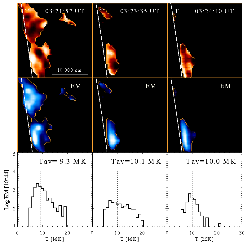
Figure 2. The maps of temperature (top row) and emission measure (middle row) for the first three times during flare rise phase (see Figure 1). The size of individual map is 30 x 30 arcsec. Brighter shades represent larger values. The corresponding quasi differential emission measure histograms (qDEM) are presented in the bottom row. The qDEM units are [cm-3/MK].
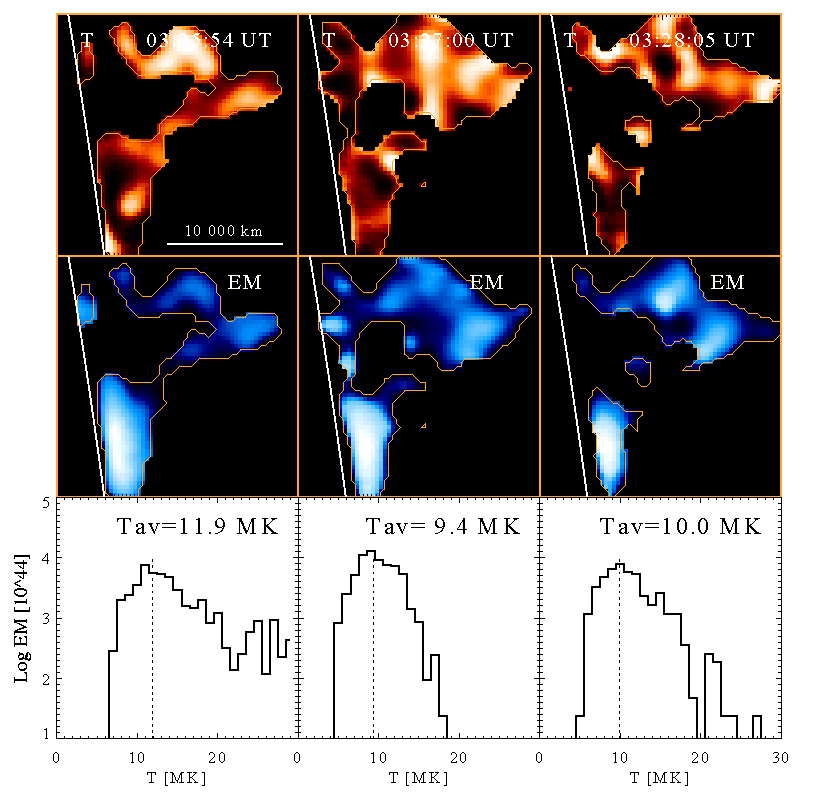
Figure 3. The same as in Figure 2 but for the three times during the flare decay phase.
3. DIFFERENTIAL EMISSION MEASURE
Our next step was to attempt to determine a "classical" differential emission measure (DEM) distribu-
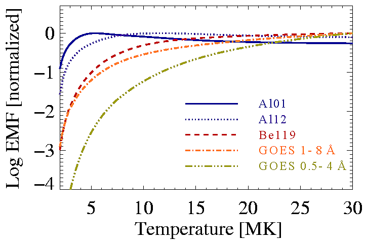
Figure 4- The emission functions for the set of five energy bands used in the calculations of differential emission measure distributions.
tions for a flare as a whole. The following data have been used as the input: GOES fluxes in the two energy bands (0.5 - 4 Å and 1 - 8 Å ) together with three flare spatially integrated fluxes observed on Yohkoh A101, A112 and Be119 images. The set of emission functions for these energy bands is presented in Figure 4. The fluxes have been calculated using corresponding SolarSoft routines and are plotted normalised, in order to better show differences in temperature behaviour. In deriving the DEM shapes we have used the classical approach and inverted the set of integral equations:
with
![]()
In this set of
equations, 'Fi is the flux measured in
line/band i, ![]() is
the corresponding emission function known from the theoretical calculations. The
is
the corresponding emission function known from the theoretical calculations. The
![]() is the unknown DEM distribution, to be found based on k observed
fluxes Fi, by solving the above set of equations. Ne and
V have their usual meaning i.e. the plasma density and the emitting
volume respectively. In order to calculate DEM distribution, we have used
Withbroe - Sylwester (WS) maximum likelihood algorithm described by Sylwester et
al., (1980). Examples of two tests showing ability of the WS technique to
recover various input models are presented in Figure 5. The input models are
plotted as thin lines, and models calculated (after 1000 iterations) are shown
as the thick lines. The first input model (left in the Figure) represents an
"isothermal" case (T =12 MK). It is seen that
the reconstructed model is much broader but the maximum of the distribution is
restored well. The representative uncertainty range is shaded. Despite the fact
that the fitted model does not exactly match synthetic input, the calculated
fluxes exactly match the input fluxes. This illustrates the ill-posed nature of
inversion problem being solved. However, if the input fluxes are systematically
biased, (as would happen for instance, in case when the GOES and SXT are
not being perfectly photometrically cross-calibrated) WS algorithm is unable to
find solution
is the unknown DEM distribution, to be found based on k observed
fluxes Fi, by solving the above set of equations. Ne and
V have their usual meaning i.e. the plasma density and the emitting
volume respectively. In order to calculate DEM distribution, we have used
Withbroe - Sylwester (WS) maximum likelihood algorithm described by Sylwester et
al., (1980). Examples of two tests showing ability of the WS technique to
recover various input models are presented in Figure 5. The input models are
plotted as thin lines, and models calculated (after 1000 iterations) are shown
as the thick lines. The first input model (left in the Figure) represents an
"isothermal" case (T =12 MK). It is seen that
the reconstructed model is much broader but the maximum of the distribution is
restored well. The representative uncertainty range is shaded. Despite the fact
that the fitted model does not exactly match synthetic input, the calculated
fluxes exactly match the input fluxes. This illustrates the ill-posed nature of
inversion problem being solved. However, if the input fluxes are systematically
biased, (as would happen for instance, in case when the GOES and SXT are
not being perfectly photometrically cross-calibrated) WS algorithm is unable to
find solution
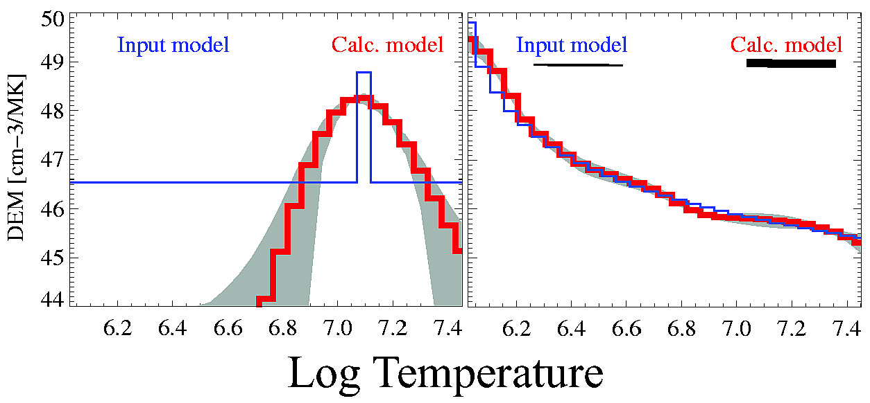
Figure 5. The results of two tests showing ability of the WS technique to recover various input models. The input models are represented by thin lines and the reconstructed distributions by the thick ones. In the left panel the single-temperature synthetic model is presented and the example model with continuous distribution of emitting plasma is shown in the right panel.
acceptable in terms of ![]() (notwithstanding of a large number of degrees of freedom). This is a
consequence of the fact that the emission functions are substantially
overlapping over the range of temperatures of interest. The second synthetic
model (right panel in Figure 5) is reconstructed much better - the input model
is represented by continuous plasma distribution. This illustrates the
regularised nature of the inversion algorithm used.
(notwithstanding of a large number of degrees of freedom). This is a
consequence of the fact that the emission functions are substantially
overlapping over the range of temperatures of interest. The second synthetic
model (right panel in Figure 5) is reconstructed much better - the input model
is represented by continuous plasma distribution. This illustrates the
regularised nature of the inversion algorithm used.
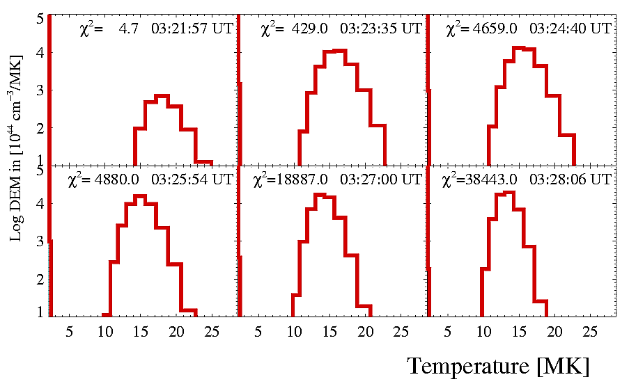
Figure 6.
The calculated differential emission measure distributions for six times
corresponding to qDEM histograms shown at the bottom of Figure 2 (top row) and 3
(bottom row) respectively. The smallest normalised ![]() value is indicated on each plot.
value is indicated on each plot.
Calculated DEM
distributions for times exactly corresponding to qDEM determinations are
displayed in Figure 6. The models presented have been obtained in the 1000th
iteration step. Large normalised ![]() values obtained indicate that the quality of
the fit is unsatisfactory. The
values obtained indicate that the quality of
the fit is unsatisfactory. The ![]() values become larger as the observed fluxes
grow and relative measurement uncertainties decrease. An inconsistency between
two approaches is evident: maxima of derived DEM and qDEM do not match each
other. (The corresponding values are ~10 MK and ~15 MK for qDEM and DEM
distributions respectively.)
values become larger as the observed fluxes
grow and relative measurement uncertainties decrease. An inconsistency between
two approaches is evident: maxima of derived DEM and qDEM do not match each
other. (The corresponding values are ~10 MK and ~15 MK for qDEM and DEM
distributions respectively.)
4. CONCLUDING REMARKS
In this research we attempted to compare the results of two independent, slightly different approaches leading to the determination of temperature distribution of plasma within flaring regions: the quasi differential emission measure distribution (qDEM) and the classical differential emission measure distribution (DEM).
In relation with the comparison of qDEM and DEM it should be stressed that qDEM distributions are determined based on the temperature and emission measure maps which have been constructed with the assumption that the flaring plasma is isothermal within a column corresponding to individual, small cross-section subpixel. The DEM distributions are calculated based on the fluxes which may contain also the non-flare emission. Especially the GOES data concern to the whole Sun. They include the quiet and active region X-ray emission which although low in comparison with the flare emission should be subtracted which is not always easy task. However, we carefully selected the event for the analysis (isolated flare) and made all conceivable corrections in order to use in the DEM calculations only these parts of total fluxes which are flare-related.
Unfortunately we were not able to resolve the problem of differential emission measure calculations of combined GOES and Yohkoh SXT observations for the C6.6 limb flare on 24 March 1993. We have found, that it is hard to obtain consistent results from a combined analysis of GOES and SXT flare integrated fluxes in terms of DEM distribution. Our conclusion is based on the fact, that the DEM reconstruction using Withbroe-Sylwester algorithm is unable to fit the observed set of flare fluxes with satisfactory quality. It appears that some unknown factors are involved in our analysis which probably influence the X-ray photometric uniformity of measurements between these two instruments as their temperature responses cover similar temperature ranges. These factors may relate to possible uncertainties in the absolute calibration of the sensitivities and/or to details of atomic physics or plasma chemical composition used in calculations of respective emission functions.
We will investigate this problem in more details based on other data sets, one example of which is the 5 October 1992 flare for which favourable SXT observations are available and qDEM analysis has been already made (Sylwester and Sylwester, 2002b).
REFERENCES
Fludra A., Sylwester J., 1986, Solar Phys. 105, 323
Sylwester J., Schrijver J., Mewe R., 1980, Solar Phys. 67, 285
Sylwester J., Sylwester B., 1998, Acta Astron. 48, 519
Sylwester J., Sylwester B., 1999, Acta Astron. 49, 189
Sylwester B., Sylwester J., 2002a, Special Publication SP-477, ed. Huguette Sawaya-Lacoste, 171
Sylwester B., Sylwester J., 2002b, Adv. Space Res. 30, in press
ACKNOWLEDGMENTS
This work has been supported by the Grant 2.P03D.024.17 of Polish Committee for Scientific Research.