In this paper, we estimate the temperature dependence of line intensities contributing to the observed features. As chlorine and potassium belongs to the group of poorly abundant elements with their respective photospheric abundances relative to H below 10-6 in the solar plasma, their emissivity has not yet been directly calculated. Therefore, we present here the results of isoelectronic sequence interpolations of the intensity vs. temperature dependence for the strong lines corresponding to 1s2 1S0 - 1s2p 1P1 ("w" line) transition in He-like ions. Results of the calculations will be useful for the final identification of the lines observed and for determination of the absolute abundance of chlorine and potassium in solar corona.
Key words: Sun, solar physics, X-ray spectroscopy, emission functions, chlorine, phosphorus and potassium.
It is of general astrophysical interest to predict spectra of hot multimillion degree
coronal plasma. A number of calculations and tabulations are presently available in this
respect. Mewe, Gronenschild and van den Oord(1985) and Mewe, Lemen and Gronenschild and
van den Oord (1986) tabulations and formulas have frequently been used in order to
synthesise spectra of coronal active regions and flares. Presently there are at least
four numerical codes available CHIANTI (Dere et al., 1997), PINTofAle (Kashyap, 2000),
XSPEC (Arnaud, 1996) for calculations of the X-ray line and continuum emissivity for
astrophysical plasma under various assumptions. However, these tables and codes
incorporate the most abundant plasma species only. Chlorine, phosphorus and potassium
line spectra are missing in all these sources. Therefore we decided to interpolate these
missing spectra of interest for us. Here we focus our attention on the strongest
transitions forming in He-like ions, which fall into the spectral region being observed
by RESIK spectrometer. The approach we have used in the interpolations can easily be
extended to the other elements and lines (papers are in preparation). We shall be
repeating this work with data from the CHIANTI code.
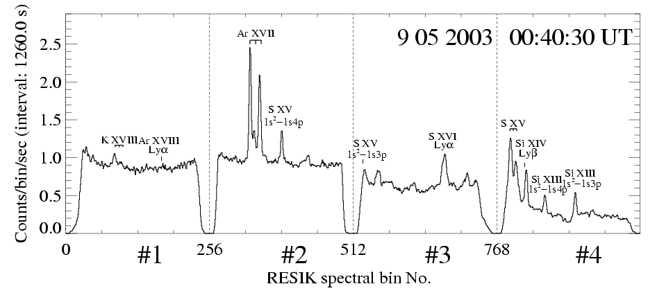
The RESIK (REntgenowsky Spektrometr s Izognutymi Kristalami) spectrometer is placed aboard CORONAS-F satellite (cf. Sylwester et al., 2003) and observes solar X-ray spectra in four channels between ~ 3.37 Å and ~ 6.08 Å. In this spectral range we observe K XVIII, Ar XVIII, Ar XVII, S XV, Si XIV, and Si XVII lines (Phillips et al., 2003). An example of a flare spectrum is shown in Fig. 1.
Figure 1: RESIK spectrum in all four channels, with stronger lines identified. The spectrum has been observed near the peak of the flare observed on 9 May 2003 at approximately 00:40 UT. Wavelength ranges are: 3.37 Å - 3.88 Å, 3.82 Å - 4.33 Å, 4.31 Å - 4.89 Å and 4.96 Å - 6.09 Å for channels 1, 2, 3 and 4 respectively. The spectrum presented has been corrected for the orbital background and the instrumental "notch" effect.
The knowledge of temperature dependence of line emissivity (called emission functions) is indispensable not only for purposes of proper line identification, but mainly for determination of elemental abundances (or their respective upper limits). For chlorine and potassium with their low solar abundances there do not appear to be available at present sufficient atomic data allowing direct calculations of line emissivity, so we performed interpolation along the He-like isoelectronic sequence in order to obtain temperature dependence of line intensities for the strongest resonance transitions ( w line in notation of Gabriel, 1972).

where R is 1 a.u., N2 is the number density (in units of cm-3) of ions excited with the electron in the upper energy level 2, A21 is the spontaneous transition probability from level 2 to the ground level. Ne and N(H) are the electron and hydrogen number densities, respectively. N(H)/Ne is the proton/electron number density ratio appropriate for a fully ionized solar plasma. N(El)/N(H) = AEl is the abundance of line parent element, Nion/N(El) is the fractional (at a given temperature) population of the ion forming the line (taken from so-called ionization balance calculations). T stands for electron temperature.
For purposes of this paper, we have used the emission function values Gi(Te) as given by Mewe et al., (1985) in the form of tabulations for elements i = Ne, Na, Mg, Al, Si, S, Ar, Ca, Fe and Ni. Respective values for P, Cl and K have been determined by means of the interpolation procedure described below. It should be noted that Mewe values have been calculated using Arnaud and Raymond (1992) ionization balance. We have found it convenient to perform interpolation along the isoelectronic sequence using normalized Gi*(T) functions, as they represent elasticities scaled to the unit elemental abundance i.e. AEl = 1.
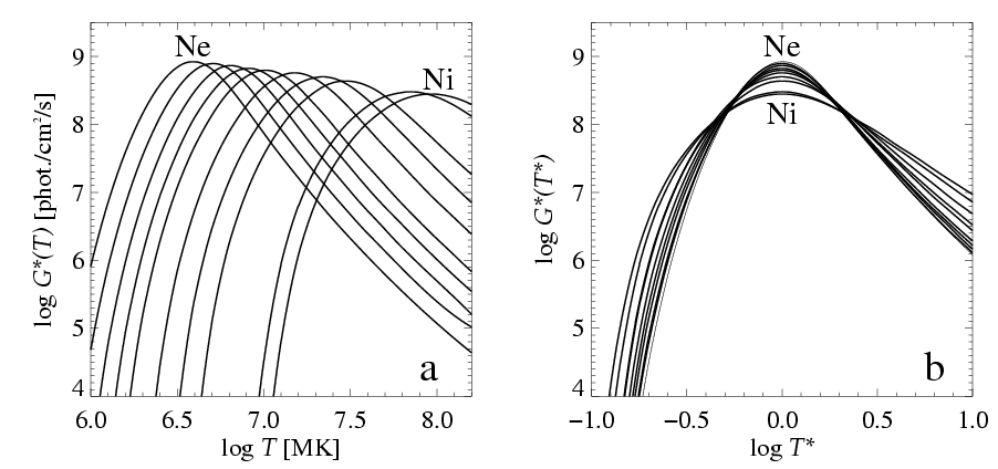
Figure 2: a) Emissivity G*(T) of the thermal plasma in w
(resonance) lines as plotted from tabulations of Mewe et al., (1985). The emissivity (per
unit elemental abundance and emission measure EM = 1048 cm-3) are plotted
for elements: Ne, Na, Mg, Al, Si, S, Ar, Ca, Fe and Ni. The curves are of similar shape.
For purpose of plotting, the emissivity have been interpolated piece by piece using
4th degree interpolation expression of the form ![]() drawn exactly through the points available from Mewe tabulations. b) When
plotted on reduced (see the text) temperature scale T*, the similarity of temperature
behaviour of emissivity curves becomes less apparent. It is seen (cf. Table 1), that the
maximum efficiency of emission depends on the atomic number.
drawn exactly through the points available from Mewe tabulations. b) When
plotted on reduced (see the text) temperature scale T*, the similarity of temperature
behaviour of emissivity curves becomes less apparent. It is seen (cf. Table 1), that the
maximum efficiency of emission depends on the atomic number.
In Fig. 2, we show Gi*(T) emissivity for the He-like w resonance transitions (1s2 1S0-1s2p 1P1) plotted against the temperature T (left) and the reduced temperature T* (right). The reduced temperature is taken as a ratio T* = T/Tm, where Tm represents the temperature where the emissivity function reaches maximum (in other words Tm represents the temperature of maximum efficiency of line formation). The systematic behaviour shown in Fig. 2 is predicted from atomic theory (Gabriel, 1972). In Table 1, we put selected characteristics of the emission function used as input for the interpolations as well as those (for P, Cl and K) obtained from the interpolation. In the Table z stands for the atomic number, T1 and T2 are the low and high temperatures at which the plasma emits at half the maximum efficiency and TFWHM is the temperature width of this temperature interval.
Table 1: Basic characteristics of emission functions for 1s2 1S0-1s2p 1P1 (w) lines of selected elements.
| Element | z | [Å] |
Tm [MK] |
log Gm* [phot/cm2/s] |
T1 T2 [MK] |
TFWHM [MK] |
| Ne | 10 | 13.4401 | 3.87 | 8.922 | 2.6 6.0 | 3.4 |
| Na | 11 | 11.0027 | 5.10 | 8.896 | 3.3 7.9 | 4.6 |
| Mg | 12 | 9.1688 | 6.43 | 8.866 | 4.2 10.1 | 5.9 |
| Al | 13 | 7.7573 | 8.24 | 8.825 | 5.2 13.0 | 7.8 |
| Si | 14 | 6.6480 | 10.28 | 8.797 | 6.4 16.5 | 10.2 |
| P+ | 15 | 5.7759 | 12.86 | 8.777 | 7.9 21.2 | 13.3 |
| S | 16 | 5.0387 | 15.07 | 8.759 | 9.2 25.5 | 16.3 |
| Cl+ | 17 | 4.4560 | 18.9 | 8.721 | 11.3 32.3 | 21.0 |
| Ar | 18 | 3.9488 | 21.98 | 8.701 | 12.6 38.0 | 25.4 |
| K+ | 19 | 3.5384 | 26.5 | 8.667 | 15.3 47.2 | 31.8 |
| Ca | 20 | 3.1773 | 29.5 | 8.639 | 16.9 54.7 | 37.8 |
| Fe | 26 | 1.8504 | 70.5 | 8.481 | 35.8 145 | 110 |
| Ni | 28 | 1.5885 | 92.0 | 8.448 | 45.7 201 | 155 |
![]() - line wavelengths are taken from CHIANTI;
- line wavelengths are taken from CHIANTI;
Gm* - value of maximum efficiency of emission [phot./cm2/s] as interpolated from Mewe et al., 1985; The uncertainty of this value is 0.01 dex
+values obtained as the results of present work.
By plotting the Tm values vs. z along the isoelectronic sequence, a clear linear dependence is noticeable.
In Fig. 3 we present respective plot for the w line. Using the least squares algorithm we draw optimum line through the points. Obtained best fit relation between the Tm and z is given by:
![]()
As the accuracy of Mewe tables extends to 3 digits (in logarithmic scale) we assume the
uncertainty of any value given in the table to be � 0.005 dex. In order to assess the uncertainty of Tm determination based on the tabulated data, we have made a Monte Carlo simulation of the dependence of Tm independently for each line, allowing every entry from Mewe table to be randomly perturbed within the rounding error (0.005 dex). The mean �1 ![]() uncertainty obtained from 100 perturbation is indicated in Figure 2a. It is important to note that the uncertainty in Tm determination is of basic importance for the accuracy of interpolation method discussed in the present paper.
uncertainty obtained from 100 perturbation is indicated in Figure 2a. It is important to note that the uncertainty in Tm determination is of basic importance for the accuracy of interpolation method discussed in the present paper.
By plotting values of G*m (from Table 1) we notice a clear dependence between G*m and z. This dependence is presented in Fig. 3b.
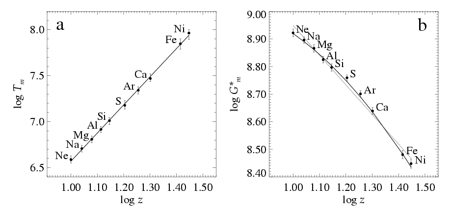
Figure 3: a) Dependence of Tm (the temperature of maximum line formation) on the atomic number z. The optimum linear fit to the points is shown (see Eq. 2 for values and uncertainties). The emission lines considered represent 1s2 1S0-1s2p 1P1 resonance (w) transition in He-like ions of Ne, Na, Mg, Al, Si, S, Ar, Ca, Fe, Ni. b) Dependence of the maximum efficiency G*m of the emission (at Tm) on the atomic number z (see Eq. 3 for values and uncertainties). The uncertainties plotted has been estimated from simple Monte Carlo simulations (see the text).
Simple linear fit is not sufficient in this case, which is easy to observe. The null-hypothesis test of the quality of the fit gives value of
With this (G*m) vs. z dependence, we observe that in general the shape of emission function can be described using the following parabolic dependence:
It is worth noting that the above parabolic relation is not only adequate to approximate the z-dependence of (G*m) at the maximum of emission efficiency i.e. where log(T*) = 0, but can also be used to approximate (G*m) vs T variations in a broader range of log(T*). This finding constitute a basis of the interpolation method adopted in the present paper.
While searching for the convenient algorithm to be used in the emission functions
interpolation, we have tested a number of other approaches including fitting with
different types of polynomials, exponential and power law formulas and orthogonal
functions. These other approaches lack the necessary generality i.e. even when we managed
to adequately fit the shape of emission function for a particular ion, we were unable to
use the same parametric form to describe emission function variation for another. Scaling
to normalized temperature T*, useful by itself, did not help in this respect. The difficulty of the present interpolation problem is probably caused by the character of
the G(T) dependence. The function is asymmetric, steeply rising by several orders of
magnitude over short interval of temperatures (due to contribution of excitation and
ionization terms) with subsequent slower decrease due to (over)ionization. Our present
approach making use of Eq. (3) appears to be flexible and accurate enough to be used in
the interpolation of such functions.
In Figure 4 we present examples of the best fitted parabolas drawn through the
"known''
points (taken from interpolated tabulated values). The lines drawn represent ''cuts''
through the optimum interpolation surface. The examples are shown for the four selected
representative values of log(T*) (indicated in each panel) from the range of interest
log(T*) ![]() [-1,1]. This range covers most part of the emission functions' variation
(i,e. by at least three orders of magnitude down from the maximum).
[-1,1]. This range covers most part of the emission functions' variation
(i,e. by at least three orders of magnitude down from the maximum).
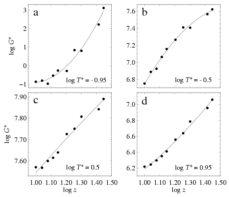
Figure 4: Plots of the ''cuts'' through optimum emission function surface for selected values of reduced temperature T*. The plots are complementary to that presented in Figure 3b and show the quality of parabolic interpolation along the isoelectronic sequence for a broad range of temperatures. It is seen that parabolic dependence (c.f. Eq. 3) is generally adequate to describe the observed G*(z)|T dependence.
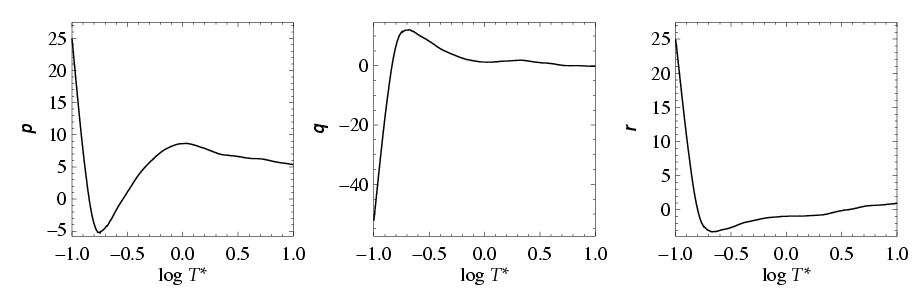
Figure 5: Plots of the temperature dependence of parameters p, q and r defining the optimum emission function surface (c.f. Eq.3). The derived uncertainties are so small that are within the width of the line plotted. [They are better shown in the respective insets as shaded areas]. The optimum emission function surface itself is shown in Figure 6.
In Figure 5, we show the z-dependence of p, q and r values defining the
"optimum interpolation surface'' together with respective formal error range
representative of the ![]() uncertainties of the fit. It is seen, that the
dependence of the best-fitted p, q and r values smoothly varies with
z. Their
formal uncertainties are rather low and can been on the blow-ups only. Therefore, the
illustrated dependencies together with Eqs (2) and (3) can be directly used in order to
predict corresponding unknown values for phosphorus, chlorine and potassium (see
Table 2). The smooth character of the p, q and r vs
log(z) behaviour allows also
for easy interpolation of existing tabulated emission function, without using the other
(formal) interpolation techniques.
uncertainties of the fit. It is seen, that the
dependence of the best-fitted p, q and r values smoothly varies with
z. Their
formal uncertainties are rather low and can been on the blow-ups only. Therefore, the
illustrated dependencies together with Eqs (2) and (3) can be directly used in order to
predict corresponding unknown values for phosphorus, chlorine and potassium (see
Table 2). The smooth character of the p, q and r vs
log(z) behaviour allows also
for easy interpolation of existing tabulated emission function, without using the other
(formal) interpolation techniques.
The overall agreement between the input data and optimum interpolation surface is presented in Figure 6, where the interpolated surface is shown (in grey) with the lines drawn on top. These lines are drawn exactly through the tabulated Mewe points and lie on the interpolation surface (to plotting accuracy).
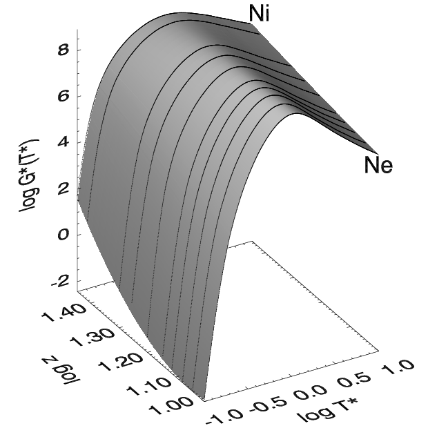
Figure 6: Interpolated emission function surface showing regular changes both in temperature and atomic number domains. The surface has been drawn using the parabolic parametric approximation (cf. Eq. 3 and Figure 4). Smooth black lines plotted on top of the surface represent these shown in Figure 2b.
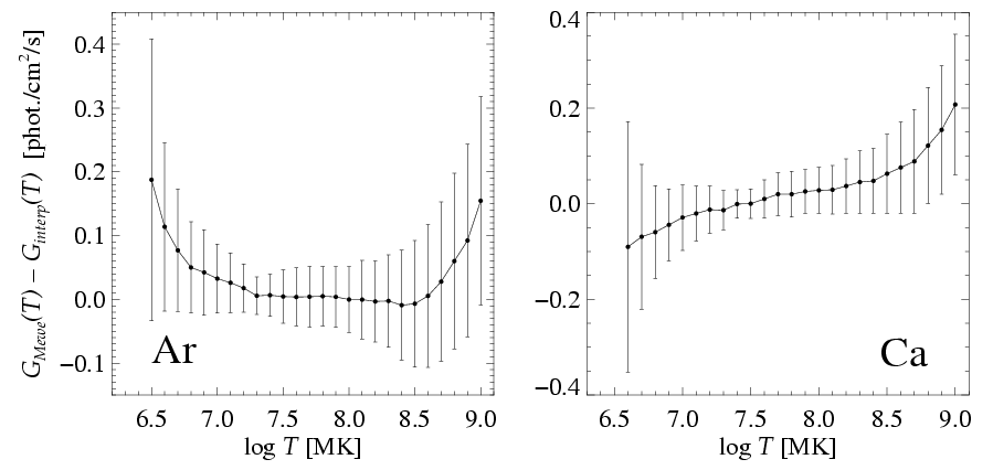
Figure 7: The interpolation consistency plot" showing the differences dex between the input tabulated values from Mewe et al. (1985) and these obtained from our interpolation. The plots are shown for two elements Ar and Ca which are the closest in the atomic number z to these of interest for us. In most cases, the observed differences are within the uncertainties of the interpolation method.
In the Figure, the differences (dex) are plotted between the tabulated and interpolated values. The temperatures for which the differences are plotted exactly correspond to these used by Mewe. The uncertainties represent values characteristic for the interpolation method, estimated assuming presence of the rounding errors (0.005 dex) in the tabulated values. It is seen from Figure 7, that the difference between the interpolated and input values are mostly negligible within the uncertainties. They are less than ~25% except towards the end of the temperature interval). This makes us confident, that the our results of the emission function interpolations will have similar level of accuracy. Therefore, we claim that the interpolated values of emission functions for P, Cl and K given in Table 2 are accurate better than 25 % over entire range of temperatures, and better than 10 % in the temperature range around the maximum efficiency of line formation. The observed differences might relate not only to the interpolation procedure itself, but also might reflect presence of uncertainties in the atomic data used for making the tabulations. In this respect, the optimum interpolation surface represents the weighted w-line emission function, averaged over the individual shapes for many elements.
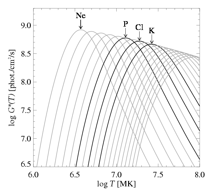
Figure 8: Comparison of the input normalized emission functions (light gray lines) with these obtained from the interpolation (black lines) as discussed in the text. Interpolated functions nicely fit into the observed pattern of variations.
In order to make the results of interpolation easy to use, we put the interpolated value in Table 2.
|
Element | 6.1 | 6.2 | 6.3 | 6.4 | 6.5 | 6.6 | 6.7 | 6.8 | 6.9 | 7.0 |
| P | - | - | 8.63 | 7.14 | 6.10 | 5.34 | 4.77 | 4.33 | 4.01 | 3.80 |
| Cl | - | - | - | 9.88 | 7.64 | 6.32 | 5.47 | 4.85 | 4.38 | 4.02 |
| K | - | - | - | - | - | - | 8.44 | 7.48 | 6.83 | 6.34 |
| Element | 7.1 | 7.2 | 7.3 | 7.4 | 7.5 | 7.6 | 7.7 | 7.8 | 7.9 | 8.0 |
| P | 3.72 | 3.78 | 3.95 | 4.21 | 4.49 | 4.78 | 5.07 | 5.34 | 5.61 | 5.86 |
| Cl | 3.76 | 3.61 | 3.58 | 3.67 | 3.86 | 4.10 | 4.37 | 4.64 | 4.90 | 5.17 |
| K | 5.97 | 5.69 | 5.52 | 5.44 | 5.47 | 5.59 | 5.79 | 6.03 | 6.28 | 6.53 |
| Element | 8.1 | 8.2 | 8.3 | 8.4 | 8.5 | 8.6 | 8.7 | 8.8 | 8.9 | 9.0 |
| P | 6.11 | 6.34 | 6.58 | 6.82 | 7.06 | 7.30 | 7.53 | 7.77 | 8.01 | 8.25 |
| Cl | 5.41 | 5.65 | 5.88 | 6.11 | 6.33 | 6.56 | 6.79 | 7.02 | 7.24 | 7.47 |
| K | 6.78 | 7.02 | 7.25 | 7.47 | 7.69 | 7.91 | 8.13 | 8.34 | 8.56 | 8.78 |
Acknowledgments.
This work has been supported by Polish KBN grants 2.P03D.024.17, 2.P03D.002.22 and PBZ-KBN-054/P03/2001. The authors wish to thank Professor Ken Phillips for reading the manuscript and helpful comments. This research was possible in part thanks to the visit exchange programme between The Royal Society and Polish Academy of Sciences.