A&A 461, 285–293 (2007)
1Astronomical Institute of Wrocław University, 51-622 Wrocław, ul. Kopernika 11, Poland
2Space Research Centre, Polish Academy of Sciences, 51-622 Wrocław, ul. Kopernika 11, Poland
ABSTRACT
Hard X-ray (HXR) emission in the footpoints of flaring loops often indicates
an asymmetry, where brighter X-ray flux usually appears in the footpoint
with a weaker magnetic field. This is explained by the fact that more
electrons can reach the chromosphere in the weaker magnetic field. However,
there are numerous exceptions to above rule, where the stronger HXR source
is located in the loop's foot that is rooted in the stronger magnetic field.
In our paper we analyse three such exceptional events from the paper by Goff
et al. (2004). For all three events, we found evidence of the magnetic loops
interactions near a brighter footpoint. Such loop interactions suggest that
for these flares the energy release is located closer to one end of the loop.
We analysed the process of electron transport in detail in the dense flaring
loop as a possible cause of the observed asymmetry. Using the flare
parameters derived from observations, we calculated how the collisional
energy losses in the loop reduce the number of electrons impacting the
chromosphere at the other footpoint. We show that these calculations
reproduce the observed flux ratios within the error limits in both
footpoints for each of the analysed events. Thus we conclude that the
injection of electrons near one of the footpoints, together with enhanced
density in the flaring loop, can explain observed HXR footpoints asymmetry.
Key words.
Observation of hard X-ray (HXR) emission in solar flares is the main key to understanding the acceleration mechanisms of particles, localization of the site of energy release, and transport effects of the non-thermal electrons. Electrons accelerated anywhere in the corona move along magnetic field lines to the chromosphere where they deposit their energy. Part of the electrons' energy is converted via the bremsstrahlung process to HXR emission. As a result, during the impulsive phase of a solar flare, double (or multiple) HXR sources are often observed at the footpoints of flaring loops, an image now widely established from the Yohkoh and RHESSI observations.
Observed HXR footpoint fluxes often show asymmetry where the brighter source is usually located in a region of the weaker photospheric magnetic field (Sakao 1994, Kundu et al. 1995, Li et al. 1997, Aschwanden et al. 1999). This asymmetry is commonly interpreted as an effect of precipitation of the non-thermal electrons in a converging magnetic field (magnetic mirror effect). In the loop's leg with a weaker magnetic field (less effective magnetic mirror), more electrons are able to reach the chromosphere and vice versa. However, there are numerous flares that do not fit the above scenario. One of five flares analysed by Sakao (1994) has a brighter footpoint located in the region of the stronger photospheric magnetic field. Asai et al. (2002) also report an example of a flare for which the brighter footpoint was found in a stronger magnetic field. Additionally, there are flares in which asymmetry changes with time. Examples of such events can be found in papers by Alexander & Metcalf (2001), Siarkowski & Falewicz (2004), and Falewicz et al. (2006).
Goff et al. (2004) studied the magnetic field strengths and hard X-ray brightness of 32 flares. They found that the brighter HXR footpoints coincide with the regions of stronger magnetic fields in 11 events. The authors designated these flares as N-type (from non-Sakao type), in contrast to S-type phenomena (for Sakao type, where a brighter footpoint is located in the region of the weaker photospheric magnetic field). According to the authors, the possible explanation of N-type events may be an asymmetry in the location of the acceleration site. If the acceleration site is located closer to the brighter footpoint, it may reduce the effects of magnetic field convergence, allowing more precipitation in this region than if the acceleration site was located at the loop apex.
Another factor that can be important for electron transport is matter density in the loop, as recently indicated e.g. by Veronig and Brown (2004). These authors report two flares observed with RHESSI for which the HXR emission comes mainly from the coronal part of the loops that are so dense as to be thick-target for electron energies up to 50 keV.
In this paper we explore the effect of the loop's density on the electron transfer in addition to an asymmetry of the injection place as the possible explanation of the Non-Sakao events. We analyse in detail three of the N-type flares studied by Goff et al. (2004) in which we have found evidence of loop interactions near the brighter of the HXR footpoints. This indicates that in these events a possible electron acceleration site may be located near one of the footpoints at the place where two magnetic loops interact. Using the observed HXR flux from an analysed flare, we calculate how the collisional energy losses reduce the number of electrons impacting the chromosphere at the other footpoint. We show that these calculations reproduce the observed flux ratios well in both footpoints for each of the analysed events.
In Sect. 2 we describe the analysed observations. The method of asymmetry modeling and calculations are presented in Sect. 3. In Sect. 4 we present the physical parameters of analysed flares. The results are discussed and we conclude in Sect. 5 and 6.
In this work we used data taken with the SXT grazing-incidence imaging telescope (Tsuneta et al.1991), the HXT Fourier synthesis telescope (Kosugi et al., 1991), and GOES broadband X-ray fluxes measured in 1-8 Ǻ and 0.5-4 Ǻ wavelength bands.
The selection of events was based on N-type flares studied by Goff et al. (2004). From Goff's list we chose three events for which the configuration of the loops observed in SXT images indicated their possible interactions close to the brighter HXR footpoints. For all three analysed events, the count rates in the L (14-23 keV), M1 (23-33 keV), and M2 (33-55 keV) channels of HXT were well above the background level during the impulsive phase. Hard X-ray images of the flares were reconstructed using the standard Pixon reconstruction procedure (Metcalf et al. 1996). We used variable accumulation times assuming a threshold count rate of 200 counts in the M2 band (33-53 keV). The main advantage of the Pixon method is that it gives superior noise suppression and accurate photometry. In one case of a weaker event, the maximum entropy method (MEM) (Gull & Daniell 1978) was used to reconstruct the image. The MEM method also works for data with small photon statistics where the Pixon method failed.
The events are described below in detail:
This event occurred on 15 March 2000 around 05:40 UT. It was a C4.0 GOES class solar flare, which started at 05:40:30 UT, reached the maximum at 05:43 UT, and ended at 06:10 UT. This flare was located near solar disc centre (W15S17).
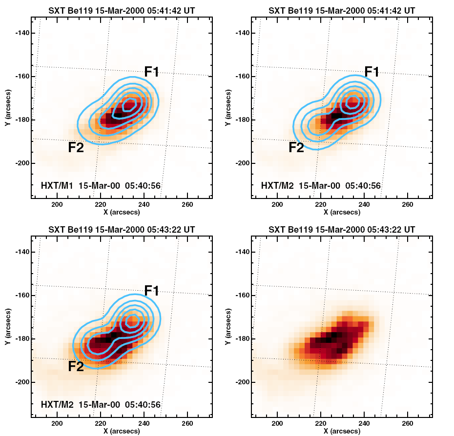
Figure 2: (Upper panel):
SXT soft X-ray image of the 15 March 2000 flare in the Be119 filter obtained at
05:41:42 UT. Contour levels at 0.1, 0.3,... 0.9 of the maximum flux show hard
X-ray images at two HXT energy ranges M1 and M2.
(Lower panel): SXT/Be119 image at 05:43:22 UT with and without the
HXT/M2 contours overlaid.
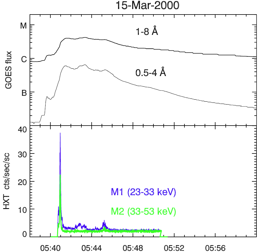
At the top of Fig. 1, GOES broadband X-ray fluxes are presented for this event measured in 1-8 Ǻ and 0.5-4 Ǻ wavelength bands. At the bottom of the same Figugure, we show hard X-ray light curves in HXT channels M1 and M2. In Fig. 2 we present SXT images at two different times around flare maximum. These images were overlaid with intensity contours in M1 and M2 channels obtained at the peak of the HXR emission. The SXT images show a small flaring loop, whereas HXR emission tends to be concentrated at each end (denoted as F1 and F2 in Fig. 2) of this loop. This concentration is more evident at higher energies (M2).
At the maximum of the HXR event ( ~ 05:42 UT), one small loop was observed in SXR (see Fig. 2 - two upper images). As the flare proceeded, a second parallel loop appeared at about 05:43 UT (see Fig. 2 - two lower images). As the presence of these two loops can be masked by HXT contours, we show the same SXT image in the lower panel of Fig. 2 with and without the HXT isocontours overlaid. The appearance of this second parallel loop is connected with a small brightening on both the SXR and HXR light curves in Fig. 1. Hard X-ray sources F1 and F2 were associated with the first SXR loop, which was the main flare loop. At lower HXR energies (channel L), emission comes generally from the F1 footpoint. Going to the higher energies (M1 and M2), the emission of the footpoints F1 and F2 dominates.
Later on during the flare decay, at least two weaker, extended loops appeared. This can be seen in Fig. 3 (left) where the composition of SXT images shows mutual locations of all loops during the flare. These extended loops lie parallel to two small loops, and the west region of their anchorage is located close to the footpoints of small loops (region A in Fig. 3 - left panel). This suggests I or Y-type interaction of the loops and we can assume that energy release in this event occurred close to the F1 footpoint of the flaring loop. This interpretation is justified by the fact that these larger loops are seen well before the flare (the last from 05:00 UT).
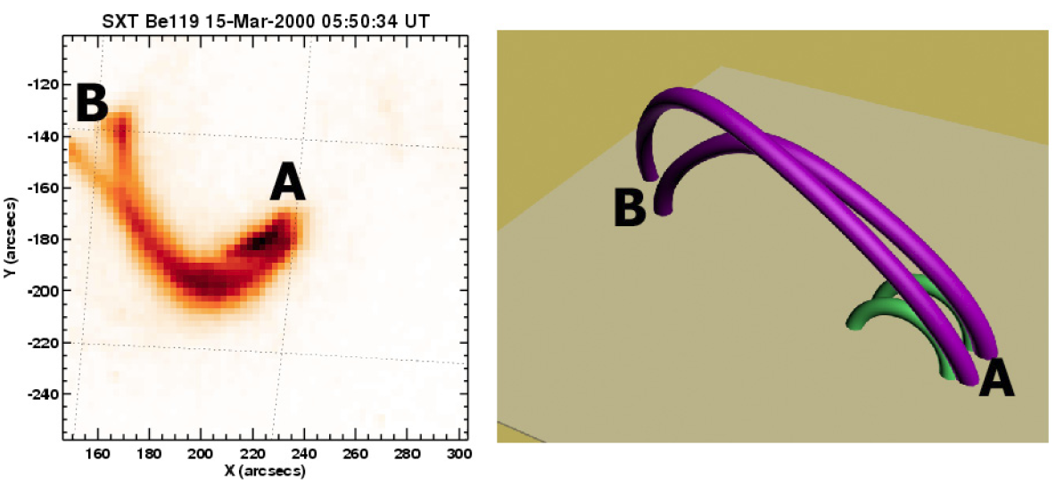
Figure 3: Left:Composition of SXT images showing mutual locations of the loops during the 15 March 2000 flare. Right: Schematic 3D models of the loop interaction in this flare. This picture was rotated and the point of view changed for clarity.
Schematic 3D models of the loop interaction in this flare is presented in the right panel of Fig. 3.
The flare on 31 August 2001 occurred at N15E37 and was an M1.6 GOES class event. It started at 10:35 UT, reached the maximum at 10:42 UT, and ended at 11:10 UT. Fig. 4 presents SXR and HXR light curves in channels M1 and M2.
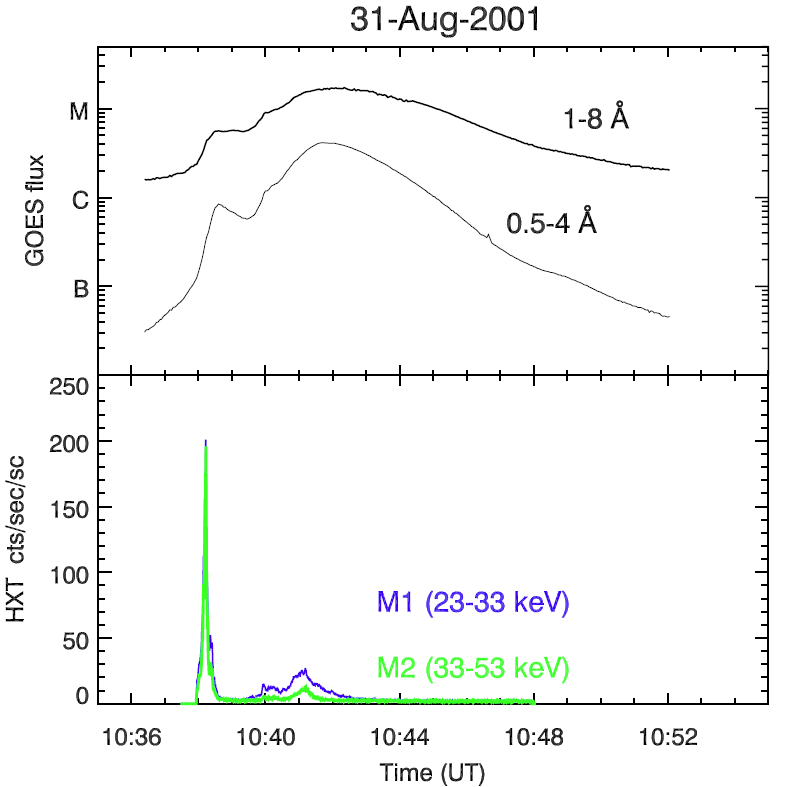
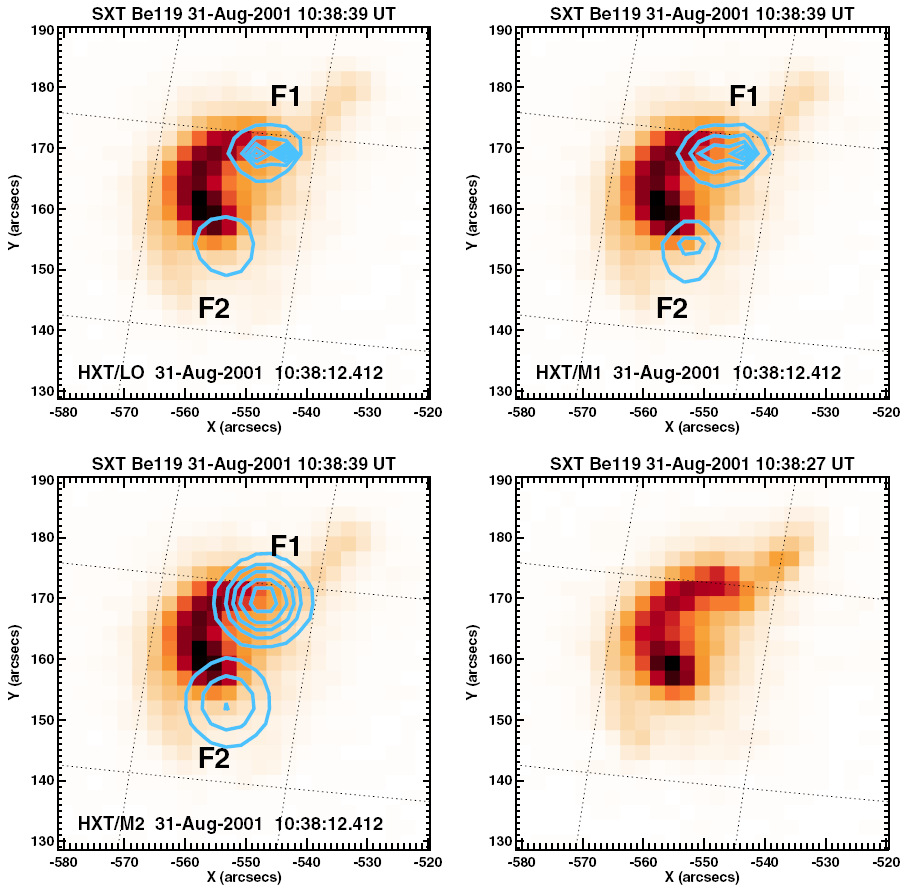
Figure 5: Soft X-ray SXT/Be119 image of the 31 August 2001 at 10:38:39 UT overplotted with iso-contours of the hard X-ray emission observed at 10:38:12 UT at three HXT energy channels: L, M1 and M2. Contour levels are 0.1, 0.3,... 0.9 of the maximum flux. The bottom right-hand corner presents an SXT/Be119 image taken at 10:38:27 UT.
In Fig. 5 we present the SXT image of this flare obtained during the rising phase at 10:38:39 UT with the Be119 filter. This image is overlaid with intensity contours obtained in LO, M1, and M2 images taken at about 10:38:12 UT. The visible sources of the hard X-ray emission can be recognised as footpoints of the magnetic loops (Falewicz et al. 2005). These footpoints denoted as F1 and F2 in Fig. 5 were connected by a loop visible in SXR.
Source F1 has two maxima in a common envelope of emission in the HXT channels LO
and M1 and probably contains also a footpoint of the another weaker loop. The
existence of this second loop was confirmed by the appearance of an extended
emission, denoted as B in Fig. 6. In the bottom right-hand corner of Fig. 5, we present an SXT/Be119 image taken at 10:38:27 UT (12 seconds earlier than the
three other). In this image the emission from the loop B is brighter and close
to an F1 footpoint. In fact a movie made of SXT images taken between 10:38:19 UT
and 10:39:09 UT clearly reveals an ejection along a loop-like shaped structure
that started exactly from source F1.
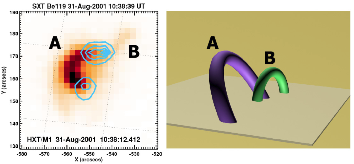
Figure 6: Left panel: Soft X-ray SXT image of the active region NOAA 9601 taken on 31 August 2001 at 10:38:39 UT. The main flaring loop, marked A, is accompanied by an extended emission, which gradually filled the shorter loop marked B. Right panel: The simple model of the interacting magnetic loops. The interaction of the loops occurred in "X" or "Y" configuration of the magnetic fields, low above the chromosphere. This picture was rotated and the point of view changed for clarity.
The observed structure of the HXR footpoints, as well as loops seen in SXR, can be explained easily with a simple model of two interacting magnetic loops. The possible spatial configuration of the loops is presented in Fig. 6 (right panel). The region of interaction of the loops was located perhaps just above the chromosphere, in the closest vicinity of the F1 footpoints (the configuration of the interacting loops was of either types X or Y), so for this flare we can assume again that the energy release took place low near the footpoint F1.
This flare occurred on 10 September 2001 around 05:13 UT. It was a C5.8 GOES class solar flare, which started at 05:12 UT, reached the maximum at 05:16 UT, and ended at 05:23 UT. The flare was located near the solar disc centre (E14 S24).
GOES and HXT light curves of the event are presented in Fig. 7. The HXT
light curves indicate that there are actually two energy release events in this
flare, one lasting from 05:13:30 UT to 05:14:00 UT and the other from 05:14:50
UT to 05:16:20 UT. This is confirmed by the sequence of SXT images in which two
nearly parallel small loops brightened one after the other during only a few
minutes.
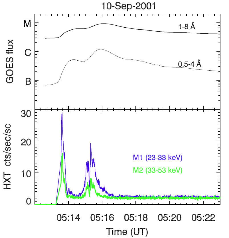
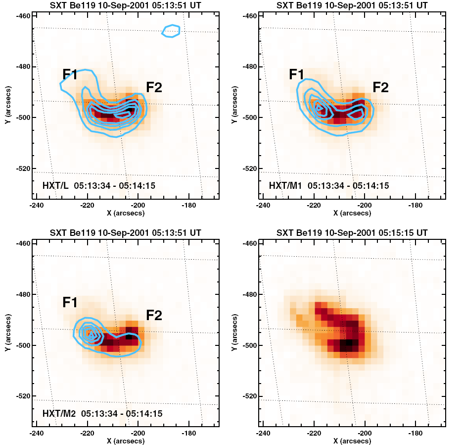
Figure 8: SXT soft X-ray images of 10 September 2001 flare at Be119 filter for two different times. Contour levels at 0.1, 0.3,... 0.9 of the maximum flux show hard X-ray images at three HXT energy ranges: L, M1, and M2. In the upper panel and the lower lefthand corner the SXT/Be119 image at 05:13:51 UT is presented when only one loop is visible. The bottom righthand corner presents an SXT/Be119 image taken at 05:15:15 UT, the time at which the first flaring loops decreased in intensity and the second one was reaching its maximum brightness.
Fig. 8 shows an SXT soft X-ray image with overlaid hard X-ray contours at three HXT energy ranges: L, M1, and M2. At lower energies (channel L), emission comes from the whole loop. Going to higher energies (M1 and M2), emission at the footpoints of this loop dominates. These footpoints are again denoted by F1 and F2 in Fig. 8.
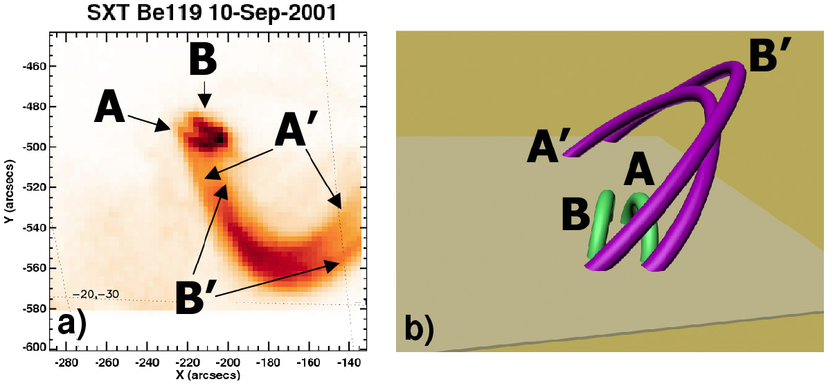
Figure 9: Left:Composition of SXT images showing mutual locations of the loops during the 10 September 2001 flare. Right: Schematic 3D models of the loops interaction for this flare. This picture was rotated and the point of view changed for clarity.
In the left panel of Fig. 9, compositions of SXT images is presented to show the mutual location of all loops during the event. The first flaring loop disappeared at about 05:15 UT (loop A), and at that time a second small parallel loop brightened (denoted as B) reaching soft X-ray flux maximum at 05:16 UT. When both small loops decreased in intensity another system of much larger loops appeared, in which two loops (denoted as A' and B') can finally be clearly distinguished. This system of loops is seen from the first SXT image, but they have a very low intensity compared to flaring loops A and B. They can also be recognised on the half and quarter resolution preflare images.
The presented image suggests the possible interaction of loop A with A' and B with B', near their F1 anchorages. Such interaction can cause energy release in the observed flare and can explain why the hard X-ray emission at the F2 footpoints of loops A and B is much weaker, if the loops are sufficiently dense to stop the non-thermal electrons on their way to these footpoints (Siarkowski & Falewicz 2005). Schematic 3D model of the loops interaction in the analysed event is presented in right panel of the Fig. 9.
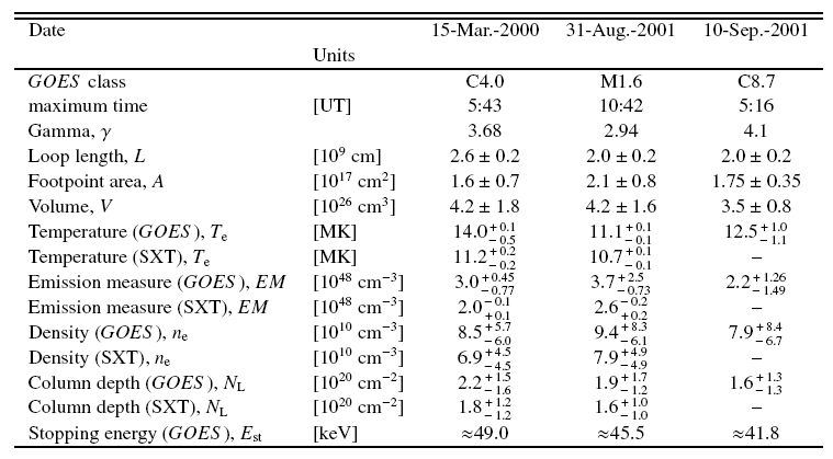
Table 1 lists the characteristics of the three events we selected. Time of
maximum for each event in Table 1 is based on GOES flux in channel 1-8 Ǻ . The
spectral slope  was
derived from the M1 and M2 HXT channel ratio. We calculated the loop length L
using the distance of centres of gravity of HXT footpoints, assuming the
semi-circular shape of the loop. When calculating L, we used the M1
channel for 10 September 2001 event and the M2 channel for two remaining flares.
The footpoint area A was calculated as the circular cross-section of the
loop seen on SXT images and volume as V=AL. We decided to use the
definition of the footpoint area from SXT images because the Pixon method gives
an accurate photometry of the sources, but the shape of reconstructed structures
is often nearly circular. Additionally the diameters of those circles usually
change with the source intensity (this can be seen for example in Fig. 5). The
values of emission measure EM, temperature T, and electron density
ne were derived using 3-second GOES data (Thomas et al., 1985)
and, for comparison, also from the SXT data for the time of HXT image during the
impulsive phase. In only one case (10-Sep-2001), we could not derive temperature
and emission measure from the SXT images because observations were unavailable
at this time (impulsive phase). For uniformity of the analysed data, we used the
GOES diagnostic that was available for all three events. Additionally
GOES data can be easily interpolated to the time where HXT images was
reconstructed. This is particularly important during the impulsive phase when
the SXT flux increases quickly. However, if possible we also calculated ne
and NL from SXT data for comparison. We calculated the column
depth NL using GOES and the SXT data as NL=ne
L. The energy of the electrons that are collisionally stopped by the
column depth is Est = (3×K ×NL)1/2
(e.g. Fisher, Canfield, and McClymont 1985), where K = 3.64 ×10⁻¹⁸ keV2 cm2. The errors given in Table 1 were
calculated using statistical uncertainties. Errors in geometrical parameters
were calculated assuming 1 pixel (2.544 arc sec) uncertainties. Our errors are
rather high, but it should be noted that we have accepted maximum errors as far
as possible for assumed geometry.
was
derived from the M1 and M2 HXT channel ratio. We calculated the loop length L
using the distance of centres of gravity of HXT footpoints, assuming the
semi-circular shape of the loop. When calculating L, we used the M1
channel for 10 September 2001 event and the M2 channel for two remaining flares.
The footpoint area A was calculated as the circular cross-section of the
loop seen on SXT images and volume as V=AL. We decided to use the
definition of the footpoint area from SXT images because the Pixon method gives
an accurate photometry of the sources, but the shape of reconstructed structures
is often nearly circular. Additionally the diameters of those circles usually
change with the source intensity (this can be seen for example in Fig. 5). The
values of emission measure EM, temperature T, and electron density
ne were derived using 3-second GOES data (Thomas et al., 1985)
and, for comparison, also from the SXT data for the time of HXT image during the
impulsive phase. In only one case (10-Sep-2001), we could not derive temperature
and emission measure from the SXT images because observations were unavailable
at this time (impulsive phase). For uniformity of the analysed data, we used the
GOES diagnostic that was available for all three events. Additionally
GOES data can be easily interpolated to the time where HXT images was
reconstructed. This is particularly important during the impulsive phase when
the SXT flux increases quickly. However, if possible we also calculated ne
and NL from SXT data for comparison. We calculated the column
depth NL using GOES and the SXT data as NL=ne
L. The energy of the electrons that are collisionally stopped by the
column depth is Est = (3×K ×NL)1/2
(e.g. Fisher, Canfield, and McClymont 1985), where K = 3.64 ×10⁻¹⁸ keV2 cm2. The errors given in Table 1 were
calculated using statistical uncertainties. Errors in geometrical parameters
were calculated assuming 1 pixel (2.544 arc sec) uncertainties. Our errors are
rather high, but it should be noted that we have accepted maximum errors as far
as possible for assumed geometry.
Usually the source of the energy release is located high in the corona and the
site of electrons injection to the flaring loop lies near the loop top (Fig. 10a). If the loop is dense enough, then electrons collisionally lose a significant
part of their energy and the emission at the footpoints Ff
will not be pure thick-target emission, but will be reduced to:
|
| (1) |
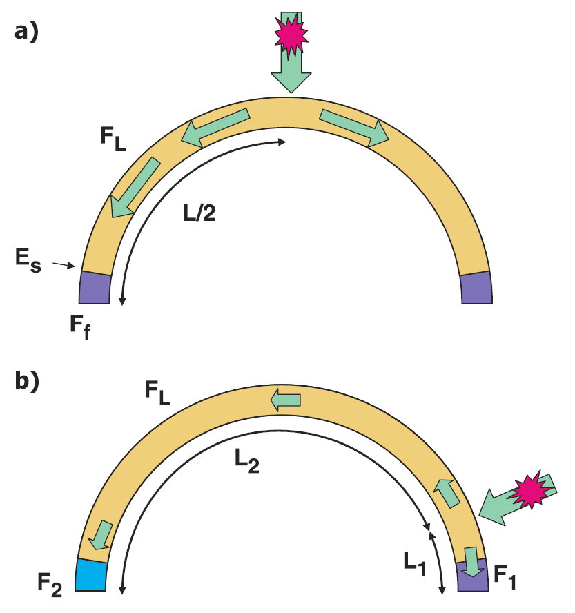
Figure 10: Schematic model of the electron transfer in the flaring loop: a) in the case where energy release is located at or above the loop apex, and b) when energy release is located near one of the footpoints. For more details see text.
The effect of collisional energy loss can be especially important in the case
where electrons are injected near one of the footpoints (Fig. 10b) as suggested
by the observations described above. Then plasma filling the loop can reduce the
number of electrons impacting the chromosphere at the other footpoint, causing
the observed HXR flux asymmetry. This model is used in the rest of the paper. We
assume that the electrons are injected in the same proportions in booth the up
and down directions along the loop and that the HXR flux (channels M1 and M2) in
the brighter footpoint F1 is a thick-target emission, i.e.: Fth
= F1 = F2 +FL
(see Eq. 1), where F1 is the flux in the brighter footpoint,
FL the flux in the whole loop legs (without footpoints;
further shortly: loop), and F2 the flux at the other footpoint.
The electrons travel from the place of injection to the footpoints F1 and
F2 along the lengths L1 and L2, respectively. Hence in our
model L1 + L2 = L, but we assume that L1 << L2
» L. To calculate F2 we adopted here an intermediate
thin-thick target model of Wheatland & Melrose (1995) in which low-energy
electrons are collisionally stopped by column depth NL = ne
L. Using the notation of Wheatland & Melrose (1995), we can write the
ratio of fluxes measured at both footpoints as
|
| (2) |
 is a photon
energy, Ec=(2KNL)1/2; K is
a function of the Coulomb logarithm (assumed as constant);
is a photon
energy, Ec=(2KNL)1/2; K is
a function of the Coulomb logarithm (assumed as constant);
 is a power-law electron
spectral index
is a power-law electron
spectral index  ), where
 is observed photon
spectral index); B(p, q) is the beta function; and
is observed photon
spectral index); B(p, q) is the beta function; and
|
| (3) |
Using an observed photon spectral index
![]() and the resulting loop's parameters ne and L, we can
calculate the flux ratio and compare it to those obtained from HXR images. Due
to the projection effect, the flux measured in footpoints F1 and F2
is not true footpoint emission but the sum of the footpoint emission and part of
the emission from the loop's legs. As the stopping energy Est
in each flaring loop is quite high (see Table 1), the emission from the legs is
important in both HXT channels M1 and M2, so the calculation of the observed
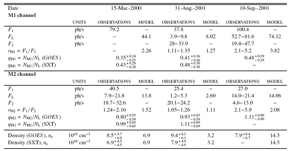
fluxes F1 and F2 values is more complicated. As the total
flare emission is a thick-target, it follows from our model that F1
= Ftotal/2 and then F2 = Ftotal/2
- FL = F1 - FL. The value FL was calculated by
evaluating the intensity near the loop top and the whole loop volume. The values
of the measured and calculated fluxes and their ratios for each of the flares
are presented in Table 2. The range of the FL values results
from the errors in the cross section of the loop. We also calculated the
stopping column depth for each energy channel, which is the column of matter in
which electrons totally rest their energy due to the collisions - only electrons
with energy E > Est can penetrate deeper. We denote
these quantities as NM1 and NM2 for channels M1 and M2 (effective
energies 29 keV and 44 keV, respectively). In Table 2 we give the ratio qM1=NM1/NL
and qM2=NM2/NL for each flare (GOES and SXT
data). For example qM2 » 0.5 means that a large fraction of electrons with energy
» 44 keV are collisionally stopped near loop's top and when qM2
³ 1.0 means that these electrons freely go to the other footpoint.
and the resulting loop's parameters ne and L, we can
calculate the flux ratio and compare it to those obtained from HXR images. Due
to the projection effect, the flux measured in footpoints F1 and F2
is not true footpoint emission but the sum of the footpoint emission and part of
the emission from the loop's legs. As the stopping energy Est
in each flaring loop is quite high (see Table 1), the emission from the legs is
important in both HXT channels M1 and M2, so the calculation of the observed
fluxes F1 and F2 values is more complicated. As the total
flare emission is a thick-target, it follows from our model that F1
= Ftotal/2 and then F2 = Ftotal/2
- FL = F1 - FL. The value FL was calculated by
evaluating the intensity near the loop top and the whole loop volume. The values
of the measured and calculated fluxes and their ratios for each of the flares
are presented in Table 2. The range of the FL values results
from the errors in the cross section of the loop. We also calculated the
stopping column depth for each energy channel, which is the column of matter in
which electrons totally rest their energy due to the collisions - only electrons
with energy E > Est can penetrate deeper. We denote
these quantities as NM1 and NM2 for channels M1 and M2 (effective
energies 29 keV and 44 keV, respectively). In Table 2 we give the ratio qM1=NM1/NL
and qM2=NM2/NL for each flare (GOES and SXT
data). For example qM2 » 0.5 means that a large fraction of electrons with energy
» 44 keV are collisionally stopped near loop's top and when qM2
³ 1.0 means that these electrons freely go to the other footpoint.
 |
The interaction of magnetic structures and conversion of magnetic free energy into plasma heating and particle acceleration is commonly regarded as the origin of solar flares. The configurations of the interacting loops observed on the Sun may be described using three main models: the I-type coalescence (interaction of two nearly parallel loops), the Y-type coalescence interacting loops (in contact only along a part of their lengths), and the X-type coalescence when some parts of two loops crossed approximately perpendicularly (Sakai and de Jager 1996). Most analyses of the observational data concerning the coalescence of loops describe the I-type interactions (e.g., Inda-Koide et al. 1995; Takahashi et al. 1996), some are related to the Y-type (e.g., Farnik et al. 1996; Hanaoka 1994), and only a few describe X-type (e.g., de Jager et al. 1995; Falewicz & Rudawy 1999; Rudawy et al. 2001). All three flares may be interpreted as resulting from the interaction of magnetic loops, as described above. Localisation of this interaction near a brighter footpoint suggests that the energy release is located low, close to one end of the loop. Using physical parameters obtained from observations and our model of the energy release near one of the footpoint, we calculated the ratio of the flux emitted by footpoints F1 and F2 (see Table 2).
For the 15 March 2000 flare, we cannot determine the observed ratio (rM1) in channel M1, but in channel M2 the obtained value (rM2) of 1.52 corresponds well to the observed range 1.24 -2.16 (see Table 2). The calculated value of ratio qM1=0.35 for the M1 channel indicates that most of electrons can reach the top of the loop only. In fact, in Fig. 2 (left panel) we can see that the emission in the M1 channel comes generally from half of the loop. In channel M2 this ratio (close to ~ 1) indicates that electrons can reach the other footpoint as can be seen also in Fig. 2 (centre and right panel). We have obtained a similar result for qM1 and qM2 for SXT data.
In the case of the 31 August 2001 event, the ratio calculated from the model of the fluxes emitted by the footpoints F1 and F2 is rM1 » 1.27 in the M1 channel and rM2 » 1.11 in the M2 channel. These values correspond very well to the observed range values 1.11 - 1.35 and 1.05 - 1.26 for the same channels (see Table 2). The calculated values of ratio qM1 for M1 channel both for GOES and SXT data indicated that most of the electrons can only reach the top of the loop (see Table 2). The calculated values qM2 (GOES and SXT data) indicate that in channel M2 the majority of electrons can reach the other footpoint.
During the 10 September 2001 flare, footpoint F2 in Fig. 8 is brighter in
channel M1 than in M2. This may be seen as contradicting the density effect, but
it should be possible for most softer spectra with a higher spectral index. In
fact for this flare,
![]() = 4.1, the higher value of all three events. It should also be remembered that
by looking at the uniform intensity loop from above we will observe more
emission at the footpoints than in the top as a projection effect.
= 4.1, the higher value of all three events. It should also be remembered that
by looking at the uniform intensity loop from above we will observe more
emission at the footpoints than in the top as a projection effect.
Using our model we obtained for M1 channel rM1 » 3.8. This last value corresponds well to the range 2.1 - 5.2 calculated from the M1 image. For the channel M2 the calculated ratio is rM2 » 2.1 and still within the observed range 2.1 -5.9.
To obtain values of the calculated ratio r=F1/F2 in the observed range, we changed the density within the error limits so that we get a best fit to the observed parameter e.g. F1, FL, and r. The adopted values of density for this and previous events are given in Table 2. As in the aforementioned cases we can observe very similar values of q (only for the GOES data because SXT data were unavailable). The calculated value of ratio qM1=0.48 for the M1 channel indicated that most of the electrons can only reach the top of the loop. In channel M2, this ratio (of ~ 1) indicates that most of the electrons can reach the other footpoint.
The values of ne, NL, qM1, and qM2 obtained from both the GOES and SXT instruments are quite similar for the first two events (see Tables 1 and 2).
All three of the flares are so-called Non-Sakao types, i.e., the HXR emission is brighter in the footpoint with a stronger underlying magnetic field. According to Goff et al. (2004) these events can be explained by an asymmetry in the location of the acceleration site. If the acceleration site is located closer to the brighter footpoint it may reduce the effects of magnetic field lines convergence over the shorter distance, allowing more precipitation in this region than if the acceleration site was located at the loop apex. However, as pointed out by the authors, there is no simple relation between the HXR flux of any individual footpoint to the magnetic flux density beneath it, so that the magnetic field strength in the footpoints can only be one of the factors that can determine asymmetry scenario. It is possible, for example, that a level of a strong field convergence, which is important for the mirroring of electrons, lies below the level where HXR emission is formed. Then, other effects, e.g. density in the loop, should be responsible for the observed asymmetry.
In fact, the densities of the analysed flaring loops are quite high, well above 1010 cm-3. Lately Veronig and Brown (2004), based on RHESSI observations, reported a new class of solar flare hard X-ray sources in which the emission is mainly in a coronal loop that is so dense as to be collisionally thick at electron energies up to » 50 keV. While the source of the energy released in these events is probably located near the loop top, both footpoints only have a weak emission.
In the analysed flares we observed evidence that the magnetic loops interact. These interactions take place low in the corona near one of the loops' anchorage, so we can assume that the region of energy release and the source of the nonthermal electrons are placed near one of the footpoints. These electrons produce observed HXR in both footpoints. However, a fraction of the electrons going to the other footpoint can be collisionally stopped in a dense loop leading to the observed asymmetry. We used the physical parameters of flaring loops obtained from GOES, SXT, and HXT observations to calculate how the density in the loop affects the number of nonthermal electrons reaching the footpoints.
Our calculations indicate that we can explain this observed asymmetry mainly as an effect of the enhanced density in the flaring loop and of the injection of electrons near one of the footpoints. We show that these calculations reproduce the observed flux ratios well in both footpoints for each of the events we analysed. However, it should be remembered that the errors of the density and loop cross-section are large, so our results are only rough estimates. Additionally, while the observed loops are small, the effects of projections are important, and a large part of the loop's emission affects the emission of the footpoints. Another topic for further discussion is that in our simple model we do not consider the changes in average pitch angle of the electrons (scattering) as they traverse the dense region. In the end, it is also very probable that there is a combination of magnetic-mirror and density effects. This last point should be especially emphasised: our density errors are sufficiently large and the magnetic field effects sufficiently unexplored. This problem needs further observations and analysis.
Acknowledgements
We are grateful to the anonymous referee for useful comments and suggestions. This work was supported by the Polish Ministry of Science and Higher Education, grants N203 022 31/2991 and 1P03D 017 29.